Copyright 2021-2024 Lawrence Livermore National Security, LLC and other MuyGPyS Project Developers. See the top-level COPYRIGHT file for details.
SPDX-License-Identifier: MIT
Univariate Regression Tutorial
This notebook walks through a simple regression workflow and explains the components of MuyGPyS.
[2]:
import numpy as np

from MuyGPyS._test.sampler import UnivariateSampler, print_results
from MuyGPyS.gp import MuyGPS
from MuyGPyS.gp.deformation import Isotropy, l2
from MuyGPyS.gp.hyperparameter import AnalyticScale, Parameter
from MuyGPyS.gp.kernels import Matern
from MuyGPyS.gp.noise import HomoscedasticNoise
from MuyGPyS.neighbors import NN_Wrapper
from MuyGPyS.optimize import Bayes_optimize
from MuyGPyS.optimize.batch import sample_batch
from MuyGPyS.optimize.loss import lool_fn
We will set a random seed here for consistency when building docs. In practice we would not fix a seed.
[3]:
np.random.seed(0)
Sampling a Curve from a Conventional GP
This notebook will use a simple one-dimensional curve sampled from a conventional Gaussian process. We will specify the domain as a grid on a one-dimensional surface and divide the observations into train and test data.
Feel free to download the source notebook and experiment with different parameters.
First we specify the region of space, the data size, and the proportion of the train/test split.
[4]:
data_count = 3000
train_ratio = 0.075
We will assume that the true data is produced with no noise, so we specify a very small noise prior for numerical stability. This is an idealized experiment with effectively no instrument error.
[5]:
nugget_noise = HomoscedasticNoise(1e-14)
We will perturb our simulated observations (the training data) with some i.i.d Gaussian measurement noise.
[6]:
measurement_noise = HomoscedasticNoise(1e-7)
Finally, we will specify kernel hyperparameters smoothness and length_scale. The length_scale scales the distances that are inputs to the kernel function, while the smoothness parameter determines how differentiable the GP prior is. The larger smoothness grows, the smoother sampled functions will become.
[7]:
sim_length_scale = Parameter(0.05)
sim_smoothness = Parameter(2.0)
We use all of these parameters to define a Matérn kernel GP and a sampler for convenience. The UnivariateSampler class is a convenience class for this tutorial, and is not a part of the library.
[8]:
sampler = UnivariateSampler(
    data_count=data_count,
    train_ratio=train_ratio,
    kernel=Matern(
        smoothness=sim_smoothness,
        deformation=Isotropy(
            l2,
            length_scale=sim_length_scale,
        ),
    ),
    noise=nugget_noise,
    measurement_noise=measurement_noise,
)
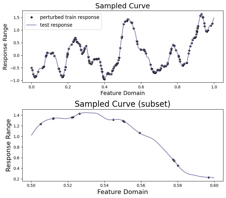
Finally, we will sample a curve from this GP prior and visualize it. Note that we perturb the train responses (the values that our model will actual receive) with Gaussian measurement noise. Further note that this is not especially fast, as sampling from a conventional Gaussian process requires computing the Cholesky decomposition of a (data_count, data_count) matrix.
[9]:
train_features, test_features = sampler.features()
[10]:
train_responses, test_responses = sampler.sample()
[11]:
sampler.plot_sample()
We will now attempt to recover the response on the held-out test data by training a univariate MuyGPS model on the perturbed training data.
Constructing Nearest Neighbor Lookups
NN_Wrapper is an api for tasking several KNN libraries with the construction of lookup indexes that empower fast training and inference. The wrapper constructor expects the training features, the number of nearest neighbors, and a method string specifying which algorithm to use, as well as any additional kwargs used by the methods. Currently supported implementations include exact KNN using
sklearn (“exact”) and approximate KNN using hnsw (“hnsw”, requires installing MuyGPyS using the hnswlib extras flag).
Here we construct an exact KNN data example with k = 30
[12]:
nn_count = 30
nbrs_lookup = NN_Wrapper(train_features, nn_count, nn_method="exact", algorithm="ball_tree")
This nbrs_lookup index is then usable to find the nearest neighbors of queries in the training data.
Sampling Batches of Data
MuyGPyS includes convenience functions for sampling batches of data from existing datasets. These batches are returned in the form of row indices, both of the sampled data as well as their nearest neighbors.
Here we sample a random batch of train_count elements. This results in using all of the train data for training. We only do that in this case because this example uses a relatively small amount of data. In practice, we would instead set batch_count to a resaonable number. In practice we find reasonable values to be in the range of 500-2000.
[13]:
batch_count = sampler.train_count
batch_indices, batch_nn_indices = sample_batch(
    nbrs_lookup, batch_count, sampler.train_count
)
These indices and nn_indices arrays are the basic operating blocks of MuyGPyS linear algebraic inference. The elements of indices.shape == (batch_count,) lists all of the row indices into train_features and train_responses corresponding to the sampled data. The rows of nn_indices.shape == (batch_count, nn_count) list the row indices into train_features and train_responses corresponding to the nearest neighbors of the sampled data.
While the user need not use the MuyGPyS.optimize.batch sampling tools to construct these data, they will need to construct similar indices into their data in order to use MuyGPyS.
Setting and Optimizing Hyperparameters
One initializes a MuyGPS object by indicating the kernel, as well as optionally specifying hyperparameters.
Consider the following example, which constructs a MuyGPs object with a Matérn kernel. The MuyGPS object expects a kernel function object, a noise noise model parameter, and a variance scale parameter. We will use an AnalyticScale instance, which has an analytic optimization method. The Matern object expects a deformation function object and a smoothness parameter. We use an isotropic deformation, so Isotropy expects a Callable indicating the metric to use (l2 distance in
this case) and a length scale parameter.
Hyperparameters can be optionally given a lower and upper optimization bound tuple on creation. If "bounds" is set, one can also set the hyperparameter value with the arguments "sample" and "log_sample" to generate a uniform or log uniform sample, respectively. Hyperparameters without optimization bounds will remain fixed during optimization.
In this experiment, we make the simplifying assumptions that we know the true length_scale and measurement_noise, and reuse the parameters used to create the sampler. We will try to learn the smoothness parameter.
[14]:
muygps = MuyGPS(
    kernel=Matern(
        smoothness=Parameter("log_sample", (0.1, 5.0)),
        deformation=Isotropy(
            l2,
            length_scale=sim_length_scale,
        ),
    ),
    noise=measurement_noise,
    scale=AnalyticScale(),
)
There is one additionally common hyperparameter, the scale variance scale parameter, that is treated differently than the others. scale cannot be directly set by the user, and always initializes to the value "unlearned". We will show how to train scale below. All hyperparameters other than scale are assumed to be fixed unless otherwise specified.
MuyGPyS depends upon linear operations on specially-constructed tensors in order to efficiently estimate GP realizations. Constructing these tensors depends upon the nearest neighbor index matrices that we described above. We can construct a distance tensor coalescing all of the square pairwise distance matrices of the nearest neighbors of a batch of points.
This snippet constructs a matrix of shape (batch_count, nn_count) coalescing all of the crosswise distances between our set of points and their nearest neighbors. This method is verbose; we will see a more concise version below.
[15]:
batch_crosswise_dists = muygps.kernel.deformation.crosswise_tensor(
    train_features,
    train_features,
    batch_indices,
    batch_nn_indices,
)
We can similarly construct a difference tensor of shape (batch_count, nn_count, nn_count) containing the pairwise distances of the nearest neighbor sets of each sampled batch element.
[16]:
pairwise_dists = muygps.kernel.deformation.pairwise_tensor(
    train_features, batch_nn_indices
)
The MuyGPS object we created earlier allows us to easily realize corresponding kernel tensors by way of its kernel function. We do not need to construct these directly for training - out optimization function will do so internally.
[17]:
Kcross = muygps.kernel(batch_crosswise_dists)
Kin = muygps.kernel(pairwise_dists)
In order to perform Gaussian process regression, we must utilize these kernel tensors in conjunction with their associated known responses. We can construct these matrices using the index matrices we derived earlier.
[18]:
batch_targets = train_responses[batch_indices]
batch_nn_targets = train_responses[batch_nn_indices]
Since we often must realize batch_targets and batch_nn_targets in close proximity to batch_crosswise_dists and batch_pairwise_dists, the MuyGPS class includes a convenience function bundles these operations.
[19]:
(
    batch_crosswise_dists,
    batch_pairwise_dists,
    batch_targets,
    batch_nn_targets,
) = muygps.make_train_tensors(
    batch_indices,
    batch_nn_indices,
    train_features,
    train_responses,
)
[20]:
Kcross = muygps.kernel(batch_crosswise_dists)
Kin = muygps.kernel(pairwise_dists)
We supply a convenient leave-one-out cross-validation utility functor class (`OptimizeFn <../MuyGPyS/gp/optimize.rst>`__) that utilizes these tensors to repeatedly realize kernel tensors during optimization. Optimization implementations are objects of this class. The library currently natively supports two optimization workflows: This optimization loop wraps a few different batch optimization methods (importable from MuyGPyS.optimize): *
`Bayes_optimize <../MuyGPyS/gp/optimize.rst>`__, which wraps `bayes_opt.BayesianOptimization <https://github.com/fmfn/BayesianOptimization>`__ in batch mode only. * `L_BFGS_B_optimize <../MuyGPyS/gp/optimize.rst>`__, which wraps the “L-BFGS-B” implementation in `scipy.optimize.minimize <https://docs.scipy.org/doc/scipy-0.18.1/reference/generated/scipy.optimize.minimize.html>`__. It is possible to create a new instance of OptimizeFn to support custom outer-loop optimizations.
This example uses Bayes_optimize. There are several additional parameters inherited from the implementation that a user might want to set. In particular, init_points (the number of “exploration” objective function evaluations to perform) and n_iter (the number of “exploitation” objective function evaluations to perform) are of use to most users. This example also sets random_state for consistency. See the documentation of
BayesianOptimization for more examples.
[21]:
muygps_optimized = Bayes_optimize(
    muygps,
    batch_targets,
    batch_nn_targets,
    batch_crosswise_dists,
    batch_pairwise_dists,
    loss_fn=lool_fn,
    verbose=True,
    random_state=1,
    init_points=5,
    n_iter=15,
)
parameters to be optimized: ['smoothness']
bounds: [[0.1 5. ]]
initial x0: [0.92898658]
|   iter    |  target   | smooth... |
-------------------------------------
| 1         | 1826.4356 | 0.9289865 |
| 2         | 2359.0765 | 2.1434078 |
| 3         | 1952.6510 | 3.6295900 |
| 4         | 614.38904 | 0.1005604 |
| 5         | 2308.5389 | 1.5814296 |
| 6         | 1707.0528 | 0.8191038 |
| 7         | 1480.1007 | 5.0       |
| 8         | 2201.4775 | 2.8303648 |
| 9         | 2373.3739 | 1.8833036 |
| 10        | 2373.2662 | 1.9964345 |
| 11        | 2374.7103 | 1.9380263 |
| 12        | 2374.7103 | 1.9379596 |
| 13        | 2374.7103 | 1.9378641 |
| 14        | 2374.7103 | 1.9377903 |
| 15        | 2374.7104 | 1.9377205 |
| 16        | 2374.7104 | 1.9376470 |
| 17        | 2374.7103 | 1.9375356 |
| 18        | 2374.6876 | 1.9448962 |
| 19        | 2374.6563 | 1.9265760 |
| 20        | 2374.6474 | 1.9497245 |
| 21        | 2374.6505 | 1.9259946 |
=====================================
As it is a variance scaling parameter that is insensitive to prediction-based optimization, we separately optimize scale. In this case, we invoke muygps.optimize_scale(), which approximates scale based upon the mean of the closed-form scale solutions associated with each of its batched nearest neighbor sets. Note that this method is sensitive to several factors, include batch_count, nn_count, and the overall size of the dataset, tending to
perform better as each of these factors increases. If we had instead used the optimization-free MuyGPyS.gp.hyperparameter.scale.Scale class, this function would effectively be a no-op and leave the value of muygps_optimized.scale unchanged.
This is usually performed after optimizing other hyperparameters.
[22]:
muygps_optimized = muygps_optimized.optimize_scale(batch_pairwise_dists, batch_nn_targets)
Inference
With set (or learned) hyperparameters, we are able to use the muygps object to predict the response of test data. Several workflows are supported.
See below a simple regression workflow, using the data structures built up in this example. This workflow uses the compact tensor-making function make_predict_tensors() to succinctly create tensors defining the pairwise_dists among each nearest neighbor set, the crosswise_dists between each test point and its nearest neighbor set, and the nn_targets or responses of the nearest neighbors in each set. We then create the Kcross cross-covariance matrix
and Kin covariance tensor and pass them to MuyGPS.posterior_mean() and MuyGPS.posterior_variance() in order to obtain our predictions.
First, we find the indices of the nearest neighbors of all of the test elements and save the results in test_nn_indices.
[23]:
test_count = test_features.shape[0]
indices = np.arange(test_count)
test_nn_indices, _ = nbrs_lookup.get_nns(test_features)
We then use nn_indices to make difference and target tensors for the test data. These tensors are similar to those used for batch optimization, except that we do not assume that we know the targets of the
[24]:
(
    test_crosswise_dists,
    test_pairwise_dists,
    test_nn_targets,
) = muygps.make_predict_tensors(
    indices,
    test_nn_indices,
    test_features,
    train_features,
    train_responses,
)
We create the kernel tensors for the optimized model.
[25]:
Kcross = muygps_optimized.kernel(test_crosswise_dists)
Kin = muygps_optimized.kernel(test_pairwise_dists)
This regression example returns predictions (posterior means) and variances for each element of the test dataset. These variances are in the form of diagonal and independent variances that encode the uncertaintainty of the model’s predictions at each test point. To scale the variances, they should be multiplied by the trained scale scaling parameters, of which there will be one scalar associated with each dimension of the response.
We use the MuyGPS.posterior_mean() and MuyGPS.posterior_variance() functions to find the posterior means and variances associated with each training prediction. The 95% confidence interval sizes are straightforward to compute as \(\sigma * 1.96\), where \(\sigma\) is the standard deviation. We compute coverage as the proportion of posterior means that differ from the true response by no more than the confidence interval size. We coverage for the 95% confidence intervals ideally
should be near 95%.
[26]:
predictions = muygps_optimized.posterior_mean(Kin, Kcross, test_nn_targets)
variances = muygps_optimized.posterior_variance(Kin, Kcross)
confidence_intervals = np.sqrt(variances) * 1.96
coverage = np.count_nonzero(np.abs(test_responses - predictions) < confidence_intervals) / test_count
Finally, we use RMSE, the mean diagonal variance and confidence interval size, as well as coverage to analyze our fit.
[27]:
print_results(
    test_responses, ("optimized", muygps_optimized, predictions, variances, confidence_intervals, coverage)
)
[27]:
| name | smoothness | length scale | noise variance | variance scale | rmse | mean variance | mean confidence interval | coverage |
|---|---|---|---|---|---|---|---|---|
| optimized | 1.937647 | 0.050000 | 0.000000 | 0.752300 | 0.016120 | 0.000239 | 0.018132 | 0.956036 |
Note here that the returned value for smoothness might be different from the smoothness used by the conventional GP. Also, the value of \(\sigma^2\) is a little different from the “true” value of 1.0. However, our mean predictions have low RMSE and our confidence intervals are low on average while our 95% confidence intervals succeed in covering ~95% of the true responses.
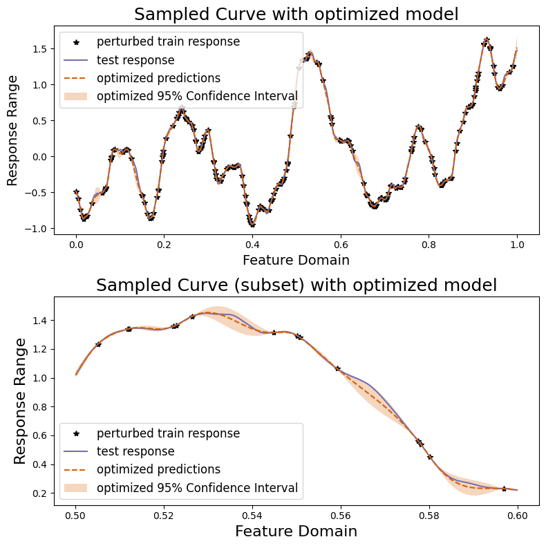
We can also plot our responses and evaluate their performance. We plot below the predicted and true curves, as well as the 95% confidence interval. We plot a smaller subset of the data in the lower curve in order to better scrutinize the 95% confidence interval.
[28]:
sampler.plot_results(("optimized", predictions, confidence_intervals))