Copyright 2021 Lawrence Livermore National Security, LLC and other MuyGPyS Project Developers. See the top-level COPYRIGHT file for details.

SPDX-License-Identifier: MIT

One-Line Regression Workflow

This notebook walks through the same regression workflow as the univariate regression tutorial.

This workflow differs from the tutorial by making use of a high-level API that automates all of the steps contained therein. MuyGPyS.examples automates a small number of such workflows. While it is recommended to stick to the lower-level API, the supported high-level APIs are useful for the simple applications that they support.

import matplotlib.pyplot as plt
import numpy as np

# This is necessary if JAX is installed as the benchmark GP is not designed with JAX in mind.
from MuyGPyS import config
config.disable_jax()

from MuyGPyS._test.gp import benchmark_sample, benchmark_sample_full, BenchmarkGP

We will set a random seed here for consistency when building docs. In practice we would not fix a seed.

np.random.seed(0)

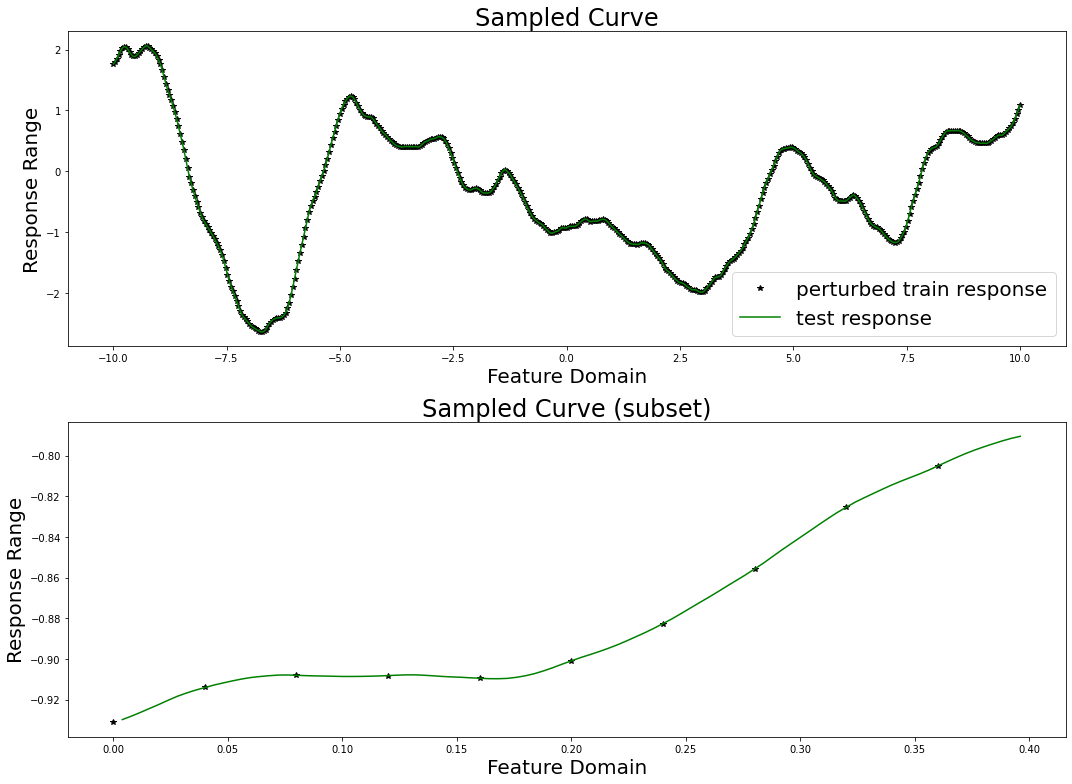
We perform the same operations to sample a curve from a conventional GP as described in the tutorial notebook.

lb = -10.0
ub = 10.0
data_count = 5001
train_step = 10
x = np.linspace(lb, ub, data_count).reshape(data_count, 1)
test_features = x[np.mod(np.arange(data_count), train_step) != 0, :]
train_features = x[::train_step, :]
test_count, _ = test_features.shape
train_count, _ = train_features.shape

nugget_var = 1e-14
fixed_length_scale = 1.0
benchmark_kwargs = {
    "kern": "matern",
    "metric": "l2",
    "eps": {"val": nugget_var},
    "nu": {"val": 2.0},
    "length_scale": {"val": fixed_length_scale},
}
gp = BenchmarkGP(**benchmark_kwargs)

y = benchmark_sample(gp, x)

test_responses = y[np.mod(np.arange(data_count), train_step) != 0, :]
measurement_eps = 1e-5
train_responses = y[::train_step, :] + np.random.normal(0, measurement_eps, size=(train_count,1))

fig, axes = plt.subplots(2, 1, figsize=(15, 11))

axes[0].set_title("Sampled Curve", fontsize=24)
axes[0].set_xlabel("Feature Domain", fontsize=20)
axes[0].set_ylabel("Response Range", fontsize=20)
axes[0].plot(train_features, train_responses, "k*", label="perturbed train response")
axes[0].plot(test_features, test_responses, "g-", label="test response")
axes[0].legend(fontsize=20)

vis_subset_size = 10
mid = int(train_count / 2)

axes[1].set_title("Sampled Curve (subset)", fontsize=24)
axes[1].set_xlabel("Feature Domain", fontsize=20)
axes[1].set_ylabel("Response Range", fontsize=20)
axes[1].plot(
    train_features[mid:mid + vis_subset_size],
    train_responses[mid:mid + vis_subset_size],
    "k*", label="perturbed train response"
)
axes[1].plot(
    test_features[mid * (train_step - 1):mid * (train_step - 1) + (vis_subset_size * (train_step - 1))],
    test_responses[mid * (train_step - 1):mid * (train_step - 1) + (vis_subset_size * (train_step - 1))],
    "g-", label="test response"
)

plt.tight_layout()

plt.show()

We now set our nearest neighbor index and kernel parameters.

nn_kwargs = {"nn_method": "exact", "algorithm": "ball_tree"}
k_kwargs = {
    "kern": "matern",
    "metric": "l2",
    "eps": {"val": measurement_eps},
    "nu": {"val": "log_sample", "bounds": (0.1, 5.0)},
    "length_scale": {"val": fixed_length_scale},
}

Finally, we run do_regress(). This function entirely instruments the regression workflow, with several tunable options. Most of the keyword arguments in this example are specified at their default values, so in practice this call need not be so verbose.

In particular, variance_mode and return_distances affect the number of returns. If variance_mode is None, then no variances variable will be returned. This is the default behavior. If return_distances is False, then no crosswise_dists or pairwise_dists tensors will be returned. This is also the default behavior.

from MuyGPyS.examples.regress import do_regress

muygps, nbrs_lookup, predictions, variances, crosswise_dists, pairwise_dists = do_regress(
    test_features,
    train_features,
    train_responses,
    nn_count=30,
    batch_count=train_count,
    loss_method="mse",
    sigma_method="analytic",
    variance_mode="diagonal",
    k_kwargs=k_kwargs,
    nn_kwargs=nn_kwargs,
    verbose=True,
    apply_sigma_sq=True,
    return_distances=True,
)

parameters to be optimized: ['nu']
bounds: [[0.1 5. ]]
initial x0: [0.49355858]
optimizer results:
      fun: 8.097389344541015e-06
 hess_inv: <1x1 LbfgsInvHessProduct with dtype=float64>
      jac: array([-6.46911389e-06])
  message: 'CONVERGENCE: NORM_OF_PROJECTED_GRADIENT_<=_PGTOL'
     nfev: 16
      nit: 7
     njev: 8
   status: 0
  success: True
        x: array([1.29131803])
Optimized sigma_sq values [0.16175717]
NN lookup creation time: 0.00046733800263609737s
batch sampling time: 0.019805562998953974s
tensor creation time: 0.008470583998132497s
hyper opt time: 5.284084254002664s
sigma_sq opt time: 0.38267214599909494s
prediction time breakdown:
        nn time:0.02363004599828855s
        agree time:7.689995982218534e-07s
        pred time:2.876988727002754s

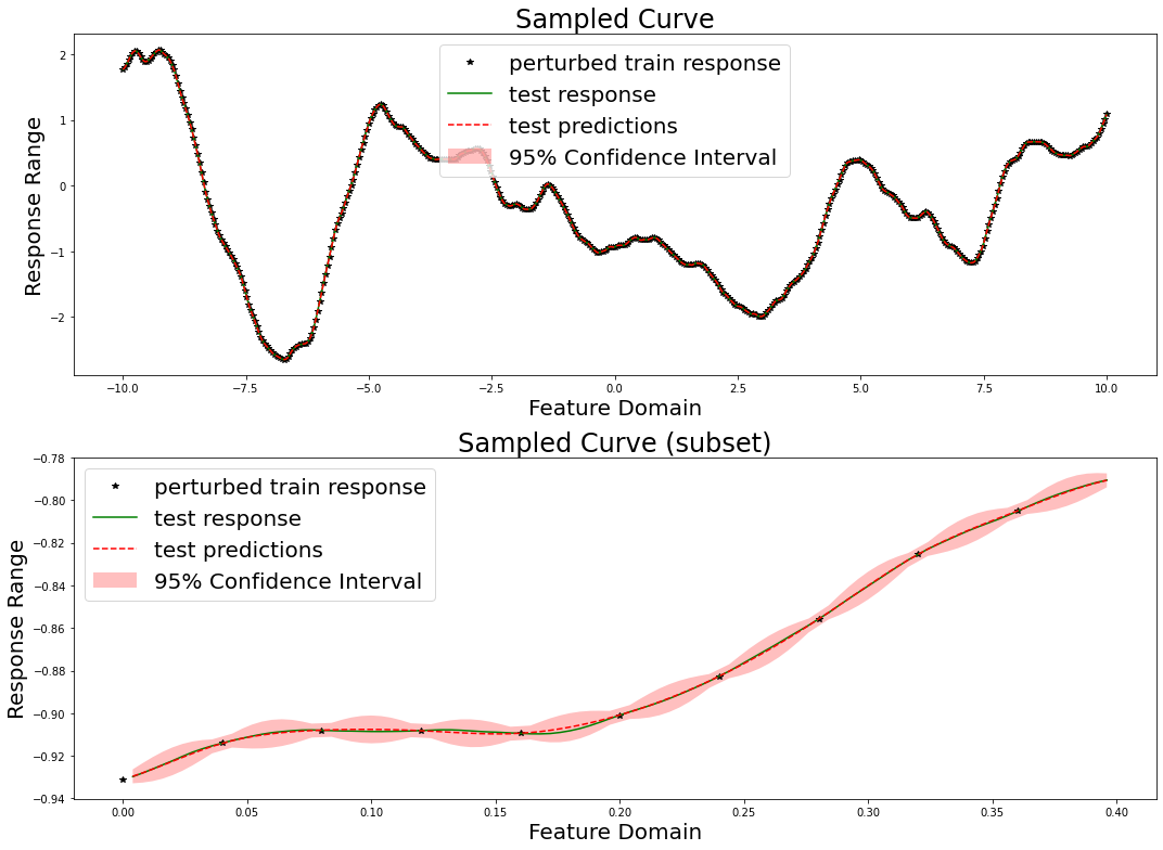
We here evaluate our prediction performance in the same manner as in the tutorial. We report the RMSE, mean diagonal posterior variance, the mean 95% confidence interval size, and the coverage, which ideally should be near 95%.

from MuyGPyS.optimize.objective import mse_fn

confidence_intervals = np.sqrt(variances) * 1.96
coverage = (
    np.count_nonzero(
        np.abs(test_responses - predictions)
        < confidence_intervals.reshape(test_count, 1)
    )
    / test_count
)
print(f"RMSE: {np.sqrt(mse_fn(predictions, test_responses))}")
print(f"mean diagonal variance: {np.mean(variances)}")
print(f"mean confidence interval size: {np.mean(confidence_intervals * 2)}")
print(f"coverage: {coverage}")

RMSE: 0.0005523047545180745
mean diagonal variance: 7.204747122314008e-06
mean confidence interval size: 0.010249195563195418
coverage: 1.0

We also produce the same plots.

fig, axes = plt.subplots(2, 1, figsize=(15, 11))

axes[0].set_title("Sampled Curve", fontsize=24)
axes[0].set_xlabel("Feature Domain", fontsize=20)
axes[0].set_ylabel("Response Range", fontsize=20)
axes[0].plot(train_features, train_responses, "k*", label="perturbed train response")
axes[0].plot(test_features, test_responses, "g-", label="test response")
axes[0].plot(test_features, predictions, "r--", label="test predictions")
axes[0].fill_between(
    test_features[:, 0],
    (predictions[:, 0] - confidence_intervals),
    (predictions[:, 0] + confidence_intervals),
    facecolor="red",
    alpha=0.25,
    label="95% Confidence Interval",
)
axes[0].legend(fontsize=20)

axes[1].set_title("Sampled Curve (subset)", fontsize=24)
axes[1].set_xlabel("Feature Domain", fontsize=20)
axes[1].set_ylabel("Response Range", fontsize=20)
axes[1].plot(
    train_features[mid:mid + vis_subset_size],
    train_responses[mid:mid + vis_subset_size],
    "k*", label="perturbed train response"
)
axes[1].plot(
    test_features[mid * (train_step - 1):mid * (train_step - 1) + (vis_subset_size * (train_step - 1))],
    test_responses[mid * (train_step - 1):mid * (train_step - 1) + (vis_subset_size * (train_step - 1))],
    "g-", label="test response"
)
axes[1].plot(
    test_features[mid * (train_step - 1):mid * (train_step - 1) + (vis_subset_size * (train_step - 1))],
    predictions[mid * (train_step - 1):mid * (train_step - 1) + (vis_subset_size * (train_step - 1))],
    "r--", label="test predictions")
axes[1].fill_between(
    test_features[mid * (train_step - 1):mid * (train_step - 1) + (vis_subset_size * (train_step - 1))][:, 0],
    (predictions[:, 0] - confidence_intervals)[mid * (train_step - 1):mid * (train_step - 1) + (vis_subset_size * (train_step - 1))],
    (predictions[:, 0] + confidence_intervals)[mid * (train_step - 1):mid * (train_step - 1) + (vis_subset_size * (train_step - 1))],
    facecolor="red",
    alpha=0.25,
    label="95% Confidence Interval",
)
axes[1].legend(fontsize=20)

plt.tight_layout()

plt.show()