SPDX-License-Identifier: MIT

Fast Regression Tutorial¶

This notebook walks through the fast regression workflow presented in Fast Gaussian Process Posterior Mean Prediction via Local Cross Validation and Precomputation (Dunton et. al 2022) and explains the relevant components of MuyGPyS.

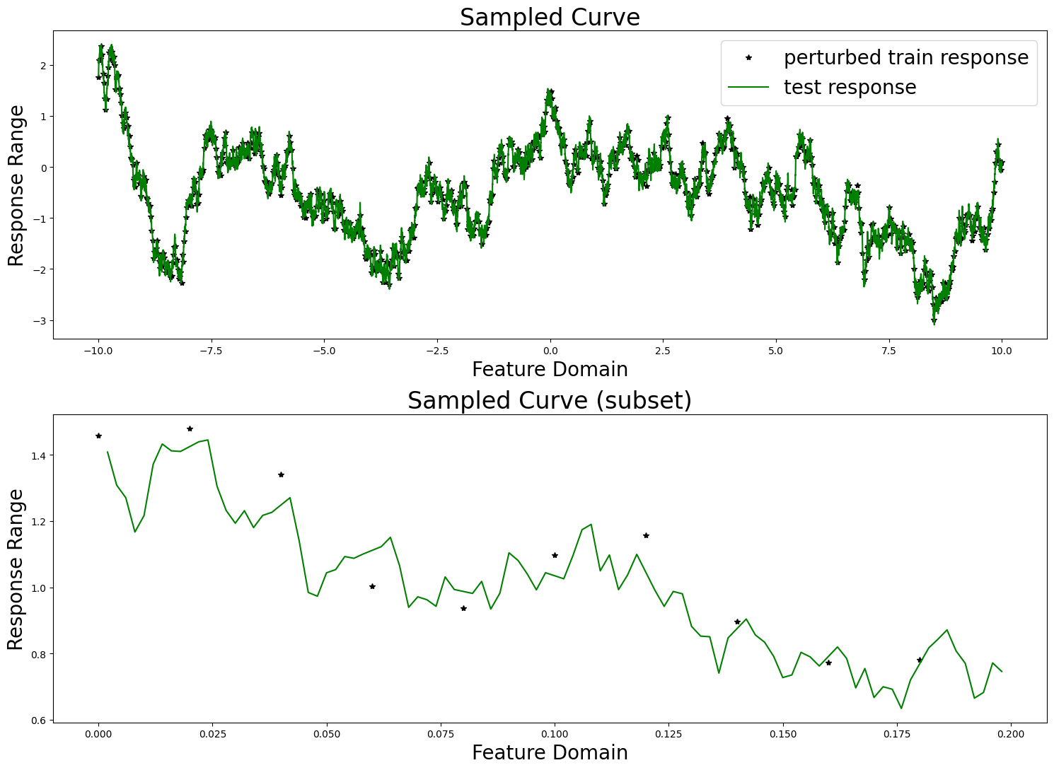
The cell below uses the same code as that found in univariate_regression_tutorial.ipynb. This includes generating the synthetic data from a GP and training two MuyGPs models to fit the data using Bayesian optimization.

[1]:

import matplotlib.pyplot as plt
import numpy as np

# This is necessary if JAX is installed as the benchmark GP is not designed with JAX in mind.
from MuyGPyS import config
if config.muygpys_jax_enabled is True:
    config.update("muygpys_jax_enabled", False)

from MuyGPyS._test.gp import benchmark_sample, benchmark_sample_full, BenchmarkGP

np.random.seed(0)

lb = -10.0
ub = 10.0
data_count = 10001
train_step = 10
x = np.linspace(lb, ub, data_count).reshape(data_count, 1)
test_features = x[np.mod(np.arange(data_count), train_step) != 0, :]
train_features = x[::train_step, :]
test_count, _ = test_features.shape
train_count, _ = train_features.shape

nugget_var = 1e-14
fixed_length_scale = 1.0
benchmark_kwargs = {
    "kern": "matern",
    "metric": "l2",
    "eps": {"val": nugget_var},
    "nu": {"val": 0.5},
    "length_scale": {"val": fixed_length_scale},
}
gp = BenchmarkGP(**benchmark_kwargs)

y = benchmark_sample(gp, x)

test_responses = y[np.mod(np.arange(data_count), train_step) != 0, :]
measurement_eps = 1e-5
train_responses = y[::train_step, :] + np.random.normal(0, measurement_eps, size=(train_count,1))
fig, axes = plt.subplots(2, 1, figsize=(15, 11))

axes[0].set_title("Sampled Curve", fontsize=24)
axes[0].set_xlabel("Feature Domain", fontsize=20)
axes[0].set_ylabel("Response Range", fontsize=20)
axes[0].plot(train_features, train_responses, "k*", label="perturbed train response")
axes[0].plot(test_features, test_responses, "g-", label="test response")
axes[0].legend(fontsize=20)

vis_subset_size = 10
mid = int(train_count / 2)

axes[1].set_title("Sampled Curve (subset)", fontsize=24)
axes[1].set_xlabel("Feature Domain", fontsize=20)
axes[1].set_ylabel("Response Range", fontsize=20)
axes[1].plot(
    train_features[mid:mid + vis_subset_size],
    train_responses[mid:mid + vis_subset_size],
    "k*", label="perturbed train response"
)
axes[1].plot(
    test_features[mid * (train_step - 1):mid * (train_step - 1) + (vis_subset_size * (train_step - 1))],
    test_responses[mid * (train_step - 1):mid * (train_step - 1) + (vis_subset_size * (train_step - 1))],
    "g-", label="test response"
)

plt.tight_layout()

plt.show()

from MuyGPyS.neighbors import NN_Wrapper
nn_count = 30
nbrs_lookup = NN_Wrapper(train_features, nn_count, nn_method="exact",algorithm="ball_tree")

from MuyGPyS.optimize.batch import sample_batch
batch_count = train_count
batch_indices, batch_nn_indices = sample_batch(
    nbrs_lookup, batch_count, train_count
)

from MuyGPyS.gp.muygps import MuyGPS
k_kwargs = {
    "kern": "matern",
    "metric": "l2",
    "eps": {"val": measurement_eps},
    #"nu": {"val": "log_sample", "bounds": (0.1, 5.0)},
    "nu": {"val": 0.5},
    #"length_scale": {"val": fixed_length_scale},
    "length_scale": {"val": "log_sample", "bounds": (0.1, 5.0)},

}
muygps = MuyGPS(**k_kwargs)

from MuyGPyS.gp.distance import crosswise_distances
batch_crosswise_dists = crosswise_distances(
    train_features,
    train_features,
    batch_indices,
    batch_nn_indices,
    metric="l2",
)

from MuyGPyS.gp.distance import pairwise_distances
pairwise_dists = pairwise_distances(
    train_features, batch_nn_indices, metric="l2"
)

Kcross = muygps.kernel(batch_crosswise_dists)
K = muygps.kernel(pairwise_dists)

batch_targets = train_responses[batch_indices, :]
batch_nn_targets = train_responses[batch_nn_indices, :]

from MuyGPyS.gp.distance import make_train_tensors
(
    batch_crosswise_dists,
    batch_pairwise_dists,
    batch_targets,
    batch_nn_targets,
) = make_train_tensors(
    muygps.kernel.metric,
    batch_indices,
    batch_nn_indices,
    train_features,
    train_responses,
)

from MuyGPyS.optimize.chassis import optimize_from_tensors


muygps = optimize_from_tensors(
    muygps,
    batch_targets,
    batch_nn_targets,
    batch_crosswise_dists,
    batch_pairwise_dists,
    loss_method="lool",
    obj_method="loo_crossval",
    opt_method="bayesian",
    verbose=False,
    random_state=1,
    init_points=5,
    n_iter=20,
)

from MuyGPyS.optimize.sigma_sq import muygps_sigma_sq_optim

K = muygps.kernel(batch_pairwise_dists)
muygps = muygps_sigma_sq_optim(muygps, batch_pairwise_dists, batch_nn_targets, sigma_method="analytic")

../_images/examples_fast_regression_tutorial_3_0.png

Fast Prediction¶

With set (or learned) hyperparameters, we are able to use the muygps object for fast prediction capability. Several workflows are supported.

See below a fast regression workflow, using the data structures built up in this example. This workflow uses the compact tensor-making function make_fast_regress_tensors() to succinctly create tensors defining the pairwise_dists among each nearest neighbor and the train_nn_targets_fast or responses of the nearest neighbors in each set. We then create theK covariance tensor and form the precomputed coefficients matrix. We then pass the precomputed coefficients matrix, the updated nn_indices matrix, and the closest neighbor of each test point to MuyGPS.fast_regress_from_indices() in order to obtain our predictions.

[2]:

from MuyGPyS.gp.distance import make_fast_regress_tensors, fast_nn_update
nn_indices,_ = nbrs_lookup.get_nns(train_features)
nn_indices = nn_indices.astype(int)

precomputed_coefficients_matrix = muygps.build_fast_regress_coeffs(
    train_features,
    nn_indices,
    train_responses)

[3]:

nn_indices = fast_nn_update(nn_indices)


test_neighbors, _ = nbrs_lookup.get_nns(test_features)
closest_neighbor = test_neighbors[:, 0]
closest_set = nn_indices[closest_neighbor, :].astype(int)

fast_predictions = muygps.fast_regress_from_indices(
    np.arange(0,test_count),
    closest_set,
    test_features,
    train_features,
    closest_neighbor,
    precomputed_coefficients_matrix)

Regular Prediction¶

With set (or learned) hyperparameters, we are able to use the muygps object to predict the response of test data. Several workflows are supported.

See below a simple regression workflow, using the data structures built up in this example. This workflow uses the compact tensor-making function make_regress_tensors() to succinctly create tensors defining the pairwise_dists among each nearest neighbor set, the crosswise_dists between each test point and its nearest neighbor set, and the nn_targets or responses of the nearest neighbors in each set. We then create the Kcross cross-covariance matrix and K covariance tensor and pass them to MuyGPS.regress() in order to obtain our predictions.

[4]:

from MuyGPyS.gp.distance import make_regress_tensors

# make the indices
test_count, _ = test_features.shape
indices = np.arange(test_count)
nn_indices, _ = nbrs_lookup.get_nns(test_features)

# make distance and target tensors
(
    crosswise_dists,
    pairwise_dists,
    nn_targets,
) = make_regress_tensors(
    muygps.kernel.metric,
    indices,
    nn_indices,
    test_features,
    train_features,
    train_responses,
)

# Make the kernel


Kcross = muygps.kernel(crosswise_dists)
K = muygps.kernel(pairwise_dists)

# perform Gaussian process regression

predictions, _ = muygps.regress(
    K,
    Kcross,
    train_responses[nn_indices, :],
    variance_mode="diagonal",
    apply_sigma_sq=True,
)

Timing Experiment¶

We compare the prediction time of a regular regression workflow to that of the fast regression workflow. In the regular regression workflow we compute the sum of the time it takes to identify the nearest neighbors of the test features, the time it takes to form the relevant kernel tensors, and the time to solve for predictions. In the fast prediction case, we compute the sum of the time it takes to identify the nearest neighbor of each test point, the coefficient lookup in the precomputed coefficient matrix, and the dot product to form predictions.

[5]:

from MuyGPyS.optimize.loss import mse_fn
import timeit


test_count, _ = test_features.shape
indices = np.arange(test_count)



def timing_regress():
    nn_indices, _ = nbrs_lookup.get_nns(test_features)
    (
        crosswise_dists,
        pairwise_dists,
        nn_targets,
    ) = make_regress_tensors(
        muygps.kernel.metric,
        indices,
        nn_indices,
        test_features,
        train_features,
        train_responses,
    )

    Kcross = muygps.kernel(crosswise_dists)
    K = muygps.kernel(pairwise_dists)
    predictions, _ = muygps.regress(
        K,
        Kcross,
        train_responses[nn_indices, :],
        variance_mode="diagonal",
        apply_sigma_sq=True,
    )

print(f"regular RMSE:")
print(f"\tRMSE: {np.sqrt(mse_fn(predictions, test_responses))}")
print("regular prediction time:")
%timeit timing_regress()



nn_indices = fast_nn_update(nn_indices)
def timing_fast_regress():
    test_neighbors, _ = nbrs_lookup.get_nns(test_features)
    closest_neighbor = test_neighbors[:, 0]
    closest_set = nn_indices[closest_neighbor, :].astype(int)

    fast_predictions = muygps.fast_regress_from_indices(
        np.arange(0,test_count),
        closest_set,
        test_features,
        train_features,
        closest_neighbor,
        precomputed_coefficients_matrix)



print(f"fast prediction RMSE:")
print(f"\tRMSE: {np.sqrt(mse_fn(np.expand_dims(fast_predictions,axis=1), test_responses))}")
print("fast prediction time:")
%timeit timing_fast_regress()

regular RMSE:
        RMSE: 0.08647726576579809
regular prediction time:
908 ms ± 7.44 ms per loop (mean ± std. dev. of 7 runs, 1 loop each)
fast prediction RMSE:
        RMSE: 0.08647708045166581
fast prediction time:
22.4 ms ± 368 µs per loop (mean ± std. dev. of 7 runs, 10 loops each)

Results¶

We achieve roughly two orders of magnitude speedup using the fast prediction acceleration. The improvement is even more dramatic when the methods are implemented in JAX.