Copyright 2021-2023 Lawrence Livermore National Security, LLC and other MuyGPyS Project Developers. See the top-level COPYRIGHT file for details.

SPDX-License-Identifier: MIT

Illustrating MuyGPs Sparsification, Prediction, and Uncertainty Quantification

This notebook illustrates how MuyGPs conditions predictions on nearest neighbors and visualizes the posterior distributions.

import matplotlib.pyplot as plt
import numpy as np

from MuyGPyS._test.sampler import UnivariateSampler2D, print_results
from MuyGPyS.gp import MuyGPS
from MuyGPyS.gp.deformation import Isotropy, l2, F2
from MuyGPyS.gp.hyperparameter import AnalyticScale, Parameter
from MuyGPyS.gp.kernels import Matern, RBF
from MuyGPyS.gp.noise import HomoscedasticNoise
from MuyGPyS.neighbors import NN_Wrapper
from MuyGPyS.optimize.batch import sample_batch

We will set a random seed here for consistency when building docs. In practice we would not fix a seed.

np.random.seed(0)

Sampling a 2D Surface from a Conventional GP

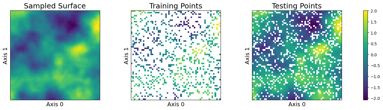
This notebook will use a simple two-dimensional curve sampled from a conventional Gaussian process. We will specify the domain as a simple grid on a one-dimensional surface and divide the observations näively into train and test data.

Feel free to download the source notebook and experiment with different parameters.

First we specify the data size and the proportion of the train/test split.

points_per_dim = 60
train_ratio = 0.2

We use all of these parameters to define a Matérn kernel GP and a sampler for convenience. The UnivariateSampler2D class is a convenience class for this tutorial, and is not a part of the library. We will use an anisotropic deformation to ensure that we sample data from the appropriate distribution.

kernel = Matern(
    smoothness=Parameter(1.5),
    deformation=Isotropy(
        l2,
        length_scale=Parameter(0.2),
    ),
)

sampler = UnivariateSampler2D(
    points_per_dim=points_per_dim,
    train_ratio=train_ratio,
    kernel=kernel,
    noise=HomoscedasticNoise(1e-7),
    measurement_noise=HomoscedasticNoise(1e-14),
)

Finally, we will sample a curve from this GP prior and visualize it. Note that we perturb the train responses (the values that our model will actual receive) with Gaussian measurement noise. Further note that this is not especially fast, as sampling from a conventional Gaussian process requires computing the Cholesky decomposition of a (data_count, data_count) matrix.

train_features, test_features = sampler.features()
train_count, _ = train_features.shape
test_count, _ = test_features.shape

train_responses, test_responses = sampler.sample()

sampler.plot_sample()

Nearest Neighbors Sparsification

MuyGPyS achieves fast posterior inference by restricting the conditioning of predictions on only the most relevant points in the training data. Currently, the library does this by utilizing the k nearest neighbors (KNN), relying upon the intution that nearby points in the input space are more highly correlated than distant points, and that nearby points contribute the overwhelming majority of the weight in the posterior mean. While methods other than nearest neighbors are also worth considering, the library presently only supports KNN.

We will illustrate the intuition behind using KNN. First, we will form a KNN index of the training data for querying. We will use the library’s built-in NN_Wrapper class, which wraps scikit-learn’s exact KNN implementation (used here) and hnswlib’s approximate but much faster and more scalable implementation.

nn_count = 50
nbrs_lookup = NN_Wrapper(train_features, nn_count, nn_method="exact", algorithm="ball_tree")

We will use the same Matérn kernel used to simulate this data.

muygps = MuyGPS(
    kernel=kernel,
    noise=HomoscedasticNoise(1e-7),
)

For a given prediction location \(\mathbf{z} \in \mathbb{R}^{d}\), and training set \(X \in \mathbb{R}^{n \times d}\) with measured univariate responses \(\mathbf{y} \in \mathbb{R}^{n}\), a conventional zero-mean GP \(f \sim \mathcal{GP}(\mathbf{0}, K(\cdot, \cdot))\) predicts the following posterior mean:

\begin{equation} E \left [ f(\mathbf{z}) \mid X, \mathbf{y} \right ] = K(\mathbf{z}, X) K(X, X)^{-1} \mathbf{y}. \end{equation}

Here \(K(\mathbf{z}, X) \in \mathbb{R}^{n}\) is the cross-covariance between \(\mathbf{z}\) and every element of the training data \(X\), and \(K(X, X) \in \mathbb{R}^{n \times n}\) is the covariance matrix of \(X\) with itself, whose inverse is sometimes called the precision matrix. The product of the cross-covariance with the precision matrix \(K(\mathbf{z}, X) K(X, X)^{-1} \in \mathbb{R}^n\) are sometimes called the kriging weights. These kriging weights effectively induce a weighted average of the observed responses \(\mathbf{y}\). Ergo, if the kriging weights are sparse (and for many practical problems they are), we need only compute the sparse elements of the kriging weights to approximate the posterior mean!

Here we will illustrate our claim by observing the kriging weights for all of the training data for a particular prediction point. We choose a test point, represented by the red plus, and plot the kriging weights of - (left) a version of the problem including all of the data (for illustration purposes) - (center) the posterior mean conditioned on the training data - (right) the posterior mean conditioned only on the nearest neighbors

test_index = int(test_count / 2) + 20

sampler.plot_kriging_weights(test_index, nbrs_lookup)

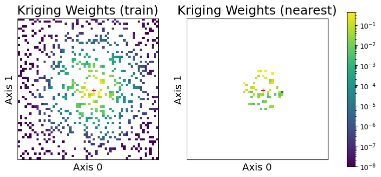
As we can see, the kriging weights of the GP problem (center plot) isolate most of the weight near the query point (red plus) in space. We can sparsify the kriging weights by only considering the nearest neighbors, represented in the right plot, while maintaining most of the covariance information to predict the point.

Comparing MuyGPs to Conventional GP Posteriors

Here we will compute posterior mean and variances for the data using both a conventional GP approach and MuyGPs.

First, we compute a conventional GP.

crosswise_dists_full = kernel.deformation.crosswise_tensor(
    test_features,
    train_features,
    np.arange(test_count),
    [np.arange(train_count) for _ in range(test_count)],
)
pairwise_dists_full = kernel.deformation.pairwise_tensor(
    train_features,
    np.arange(train_count),
)

Kcross_full = kernel(crosswise_dists_full)
Kin_full = kernel(pairwise_dists_full)

Here we’ll stop to note that we have three matrices: the cross-covariance (Kcross_full), the covariance (Kin_full), and the response vector (train_responses). The mean and covariance are computed in terms of dense solves involving these matrices, whose dimensions increase linearly in the data size (resulting in a quadratic increase in storage and a cubic increase in runtime).

print(f"Kcross_full shape: {Kcross_full.shape}")
print(f"Kin_full shape: {Kin_full.shape}")
print(f"train_responses shape: {train_responses.shape}")

Kcross_full shape: (2880, 720)
Kin_full shape: (720, 720)
train_responses shape: (720,)

We use these matrices to compute the posterior mean and variance, and construct univariate 95% confidence intervals for each individual prediction.

mean_full = Kcross_full @ np.linalg.solve(Kin_full, train_responses)
covariance_full = 1 - Kcross_full @ np.linalg.solve(Kin_full, Kcross_full.T)
covariance_diag = np.diag(covariance_full)
confidence_interval_full = np.sqrt(covariance_diag) * 1.96
coverage_full = (
    np.count_nonzero(
        np.abs(test_responses - mean_full) < confidence_interval_full
    ) / test_count
)

Now we repeat a similar workflow for MuyGPs. This time, we sample nearest neighbors from the previously-constructed index and create distance tensors using MuyGPyS convenience functions.

nn_indices, _ = nbrs_lookup.get_nns(test_features)
(
    crosswise_dists,
    pairwise_dists,
    nn_responses,
) = muygps.make_predict_tensors(
    np.arange(test_count),
    nn_indices,
    test_features,
    train_features,
    train_responses,
)

Kcross = muygps.kernel(crosswise_dists)
Kin = muygps.kernel(pairwise_dists)

We now have three tensors, similar to the conventional workflow: Kcross, Kin, and nn_responses. These tensors have the following shapes, which only increase linearly as the data size increases, which drastically improves scalability compared to the conventional GP.

print(f"Kcross shape: {Kcross.shape}")
print(f"Kin shape: {Kin.shape}")
print(f"nn_responses shape: {nn_responses.shape}")

Kcross shape: (2880, 50)
Kin shape: (2880, 50, 50)
nn_responses shape: (2880, 50)

Here we use MuyGPyS to compute the posterior distribution, similar in form to the conventional GP.

mean_muygps = muygps.posterior_mean(
    Kin, Kcross, nn_responses
)
variance_muygps = muygps.posterior_variance(
    Kin, Kcross
)
confidence_interval_muygps = np.sqrt(variance_muygps) * 1.96
coverage_muygps = (
    np.count_nonzero(
        np.abs(test_responses - mean_muygps) < confidence_interval_muygps
    ) / test_count
)

Finally, we compare our performance. The left column plots the absolute residual of each posterior mean implementation with the true response for the whole test dataset. The center column plots the size of the 95% confidence intervals across the whole dataset. Finally, the right column plots where the residual exceeds the confidence interval. Red points in the right column exceed the confidence interval, which should comprise 5% of the data if the uncertainties are calibrated.

sampler.plot_errors(
    ("MuyGPs", mean_muygps, confidence_interval_muygps),
    ("Conventional", mean_full, confidence_interval_full),
)

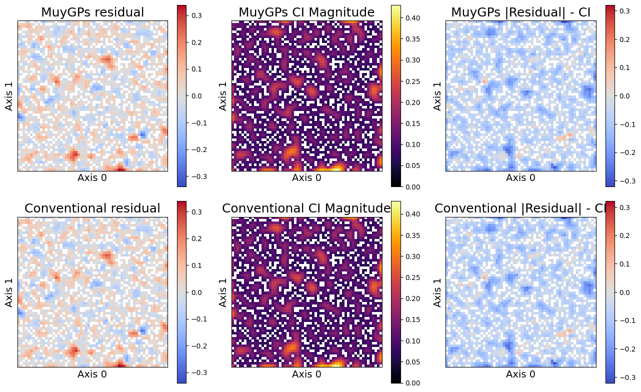
We can see that the MuyGPyS posteriors closely matches the conventional GP, while remaining much more scalable. Note especially that the same points exceed the confidence interval for each model. Hopefully, this demonstration has helped to motivate the MuyGPs sparsification approach. For more validation, we directly compare some summary statistics of the two approaches.

print_results(
    test_responses,
    ("MuyGPyS", muygps, mean_muygps, variance_muygps, confidence_interval_muygps, coverage_muygps),
    ("Conventional", muygps, mean_full, covariance_diag, confidence_interval_full, coverage_full),
)

name	smoothness	length scale	noise variance	variance scale	rmse	mean variance	mean confidence interval	coverage
MuyGPyS	1.500000	0.200000	0.000000	1.000000	0.061744	0.004271	0.118239	0.950347
Conventional	1.500000	0.200000	0.000000	1.000000	0.061740	0.004269	0.118214	0.950347