SPDX-License-Identifier: MIT

Univariate Regression Tutorial¶

This notebook walks through a simple regression workflow and explains the componenets of MuyGPyS.

[1]:

import matplotlib.pyplot as plt
import numpy as np

from MuyGPyS.testing.gp import benchmark_sample, benchmark_sample_full, BenchmarkGP

We will set a random seed here for consistency when building docs. In practice we would not fix a seed.

[2]:

np.random.seed(0)

Sampling a Curve from a Conventional GP¶

This notebook will use a simple one-dimensional curve sampled from a conventional Gaussian process. The Gaussian process in question is implemented in MuyGPyS.testing.gp.BenchmarkGP. It is intended for testing purposes only. We will specify the domain as a grid on a one-dimensional surface and divide the observations into train and test data. Feel free to experiment with different parameters.

[3]:

lb = -10.0
ub = 10.0
data_count = 10001
train_step = 10
x = np.linspace(lb, ub, data_count).reshape(data_count, 1)
test_features = x[np.mod(np.arange(data_count), train_step) != 0, :]
train_features = x[::train_step, :]
test_count, _ = test_features.shape
train_count, _ = train_features.shape

We will now define a Matern kernel function and create a conventional GP. Note here that we are setting a small value for eps, the prior variance of the “nugget” or diagonal noise matrix added to the raw kernel matrix to a small value purely for numerical stability. This is an idealized experiment with no instrument error.

[4]:

nugget_var = 1e-14
fixed_length_scale = 1.0
benchmark_kwargs = {
    "kern": "matern",
    "metric": "l2",
    "eps": {"val": nugget_var},
    "nu": {"val": 2.0},
    "length_scale": {"val": fixed_length_scale},
}
gp = BenchmarkGP(**benchmark_kwargs)

Finally, we will sample a curve from this GP prior and visualize it. Note that we perturb the train responses (the values that our model will actual receive) with Gaussian measurement noise. Further note that this is not especially fast, as sampling from a conventional Gaussian process requires computing the Cholesky decomposition of a (data_count, data_count) matrix.

[5]:

y = benchmark_sample(gp, x)

[6]:

test_responses = y[np.mod(np.arange(data_count), train_step) != 0, :]
measurement_eps = 1e-5
train_responses = y[::train_step, :] + np.random.normal(0, measurement_eps, size=(train_count,1))

[7]:

fig, axes = plt.subplots(2, 1, figsize=(15, 11))

axes[0].set_title("Sampled Curve", fontsize=24)
axes[0].set_xlabel("Feature Domain", fontsize=20)
axes[0].set_ylabel("Response Range", fontsize=20)
axes[0].plot(train_features, train_responses, "k*", label="perturbed train response")
axes[0].plot(test_features, test_responses, "g-", label="test response")
axes[0].legend(fontsize=20)

vis_subset_size = 10
mid = int(train_count / 2)

axes[1].set_title("Sampled Curve (subset)", fontsize=24)
axes[1].set_xlabel("Feature Domain", fontsize=20)
axes[1].set_ylabel("Response Range", fontsize=20)
axes[1].plot(
    train_features[mid:mid + vis_subset_size],
    train_responses[mid:mid + vis_subset_size],
    "k*", label="perturbed train response"
)
axes[1].plot(
    test_features[mid * (train_step - 1):mid * (train_step - 1) + (vis_subset_size * (train_step - 1))],
    test_responses[mid * (train_step - 1):mid * (train_step - 1) + (vis_subset_size * (train_step - 1))],
    "g-", label="test response"
)

plt.tight_layout()

plt.show()

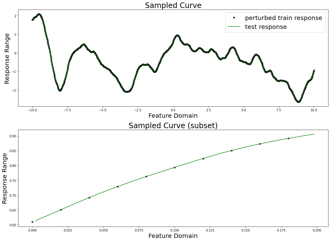
../_images/examples_univariate_regression_tutorial_12_0.png

We will now attempt to recover the response on the held-out test data by training a univariate MuyGPS model on the perturbed training data.

Constructing Nearest Neighbor Lookups¶

NN_Wrapper is an api for tasking several KNN libraries with the construction of lookup indexes that empower fast training and inference. The wrapper constructor expects the training features, the number of nearest neighbors, and a method string specifying which algorithm to use, as well as any additional kwargs used by the methods. Currently supported implementations include exact KNN using sklearn (“exact”) and approximate KNN using hnsw (“hnsw”).

Here we construct an exact KNN data example with k = 30

[8]:

from MuyGPyS.neighbors import NN_Wrapper
nn_count = 30
nbrs_lookup = NN_Wrapper(train_features, nn_count, nn_method="exact", algorithm="ball_tree")

This nbrs_lookup index is then usable to find the nearest neighbors of queries in the training data.

Sampling Batches of Data¶

MuyGPyS includes convenience functions for sampling batches of data from existing datasets. These batches are returned in the form of row indices, both of the sampled data as well as their nearest neighbors.

Here we sample a random batch of train_count elements. This results in using all of the train data for training. We only do that in this case because this example uses a relatively small amount of data. In practice, we would instead set batch_count to a resaonable number. In practice we find reasonable values to be in the range of 500-2000.

[9]:

from MuyGPyS.optimize.batch import sample_batch
batch_count = train_count
batch_indices, batch_nn_indices = sample_batch(
    nbrs_lookup, batch_count, train_count
)

These indices and nn_indices arrays are the basic operating blocks of MuyGPyS linear algebraic inference. The elements of indices.shape == (batch_count,) lists all of the row indices into train_features and train_responses corresponding to the sampled data. The rows of nn_indices.shape == (batch_count, nn_count) list the row indices into train_features and train_responses corresponding to the nearest neighbors of the sampled data.

While the user need not use the MuyGPyS.optimize.batch sampling tools to construct these data, they will need to construct similar indices into their data in order to use MuyGPyS.

Setting and Optimizing Hyperparameters¶

One initializes a MuyGPS object by indicating the kernel, as well as optionally specifying hyperparameters.

Consider the following example, which constructs a Matern kernel with all parameters fixed aside from "nu" and "sigma_sq". Note that we are here making the simplifying assumtions that we know the true length_scale and measurement error.

[10]:

from MuyGPyS.gp.muygps import MuyGPS
k_kwargs = {
    "kern": "matern",
    "metric": "l2",
    "eps": {"val": measurement_eps},
    "nu": {"val": "log_sample", "bounds": (0.1, 5.0)},
    "length_scale": {"val": fixed_length_scale},
}
muygps = MuyGPS(**k_kwargs)

Hyperparameters can be initialized or reset using dictionary arguments containing the optional "val" and "bounds" keys. "val" sets the hyperparameter to the given value, and "bounds" determines the upper and lower bounds to be used for optimization. If "bounds" is set, "val" can also take the arguments "sample" and "log_sample" to generate a uniform or log uniform sample, respectively. If "bounds" is set to "fixed", the hyperparameter will remain fixed during any optimization. This is the default behavior for all hyperparameters if "bounds" is unset by the user.

One sets the model hyperparameter eps, as well as kernel-specific hyperparameters, e.g. nu and length_scale for the Matern kernel, at initialization as above.

There is one common hyperparameter, the sigma_sq scale parameter, that violates these rules. sigma_sq cannot be directly set by the user, and always initializes to the value "unlearned". We will show how to train sigma_sq below. All hyperparameters other than sigma_sq are assumed to be fixed unless otherwise specified.

MuyGPyS depends upon linear operations on specially-constructed tensors in order to efficiently estimate GP realizations. Constructing these tensors depends upon the nearest neighbor index matrices that we described above. We can construct a distance tensor coalescing all of the square pairwise distance matrices of the nearest neighbors of a batch of points.

This snippet constructs a matrix of shape (batch_count, nn_count) coalescing all of the distance vectors between the same batch of points and their nearest neighbors.

[11]:

from MuyGPyS.gp.distance import crosswise_distances
crosswise_dists = crosswise_distances(
    train_features,
    train_features,
    batch_indices,
    batch_nn_indices,
    metric="l2",
)

We can similarly construct a Euclidean distance tensor of shape (batch_count, nn_count, nn_count) containing the pairwise distances of the nearest neighbor sets of each sampled batch element.

[12]:

from MuyGPyS.gp.distance import pairwise_distances
pairwise_dists = pairwise_distances(
    train_features, batch_nn_indices, metric="l2"
)

The MuyGPS object we created earlier allows us to easily realize kernel tensors by way of its kernel function.

[13]:

Kcross = muygps.kernel(crosswise_dists)
K = muygps.kernel(pairwise_dists)

In order to perform Gaussian process regression, we must utilize these kernel tensors in conjunction with their associated known responses. We can construct these matrices using the index matrices we derived earlier.

[14]:

batch_targets = train_responses[batch_indices, :]
batch_nn_targets = train_responses[batch_nn_indices, :]

Since we often must realize batch_targets and batch_nn_targets in close proximity to crosswise_dists and pairwise_dists, the library includes a convenience function make_train_tensors() that bundles these operations.

[15]:

from MuyGPyS.gp.distance import make_train_tensors
(
    crosswise_dists,
    pairwise_dists,
    batch_targets,
    nn_targets,
) = make_train_tensors(
    muygps.kernel.metric,
    batch_indices,
    batch_nn_indices,
    train_features,
    train_responses,
)

We supply a convenient leave-one-out cross-validation utility that utilizes the crosswise_dists and pairwise_dists tensors to repeatedly realize kernel tensors during optimization.

[16]:

from MuyGPyS.optimize.chassis import scipy_optimize_from_tensors
scipy_optimize_from_tensors(
    muygps,
    batch_targets,
    batch_nn_targets,
    crosswise_dists,
    pairwise_dists,
    loss_method="mse",
    verbose=True,
)

parameters to be optimized: ['nu']
bounds: [[0.1 5. ]]
initial x0: [2.28105771]
optimizer results:
      fun: 3.699544025744407e-06
 hess_inv: <1x1 LbfgsInvHessProduct with dtype=float64>
      jac: array([9.28648777e-06])
  message: b'CONVERGENCE: NORM_OF_PROJECTED_GRADIENT_<=_PGTOL'
     nfev: 2
      nit: 0
   status: 0
  success: True
        x: array([2.28105771])

[16]:

array([2.28105771])

Note here that the returned value for nu might be different from the nu used by the conventional GP.

If you do not need to retain the distances tensors or batch targets for future reference, you can use a related function that realizes them internally.

[17]:

# from MuyGPyS.optimize.chassis import scipy_optimize_from_indices
# scipy_optimize_from_indices(
#     muygps,
#     batch_indices,
#     batch_nn_indices,
#     train_features,
#     train_responses,
#     loss_method="mse",
#     verbose=False,
# )

As it is a variance scaling parameter that is insensitive to prediction-based optimization, we separately optimize sigma_sq. In this case, we invoke MuyGPS.sigma_sq_optim(), which approximates sigma_sq based upon the mean of the closed-form sigma_sq solutions associated with each of its batched nearest neighbor sets. Note that this method is sensitive to several factors, include batch_count, nn_count, and the overall size of the dataset, tending to perform better as each of these factors increases.

This is usually performed after optimizing other hyperparameters.

[18]:

K = muygps.kernel(pairwise_dists)
muygps.sigma_sq_optim(K, batch_nn_indices, train_responses)

[18]:

array([0.63772583])

Inference¶

With set (or learned) hyperparameters, we are able to use the muygps object to predict the response of test data. Several workflows are supported.

See below a simple regression workflow, using the data structures built up in this example. This workflow uses the compact tensor-making function make_regress_tensors() to succinctly create tensors defining the pairwise_dists among each nearest neighbor set, the crosswise_dists between each test point and its nearest neighbor set, and the nn_targets or responses of the nearest neighbors in each set. We then create the Kcross cross-covariance matrix and K covariance tensor and pass them to MuyGPS.regress() in order to obtain our predictions.

[19]:

from MuyGPyS.gp.distance import make_regress_tensors

# make the indices
test_count, _ = test_features.shape
indices = np.arange(test_count)
nn_indices, _ = nbrs_lookup.get_nns(test_features)

# make distance and target tensors
(
    crosswise_dists,
    pairwise_dists,
    nn_targets,
) = make_regress_tensors(
    muygps.kernel.metric,
    indices,
    nn_indices,
    test_features,
    train_features,
    train_responses,
)

# Make the kernels
Kcross = muygps.kernel(crosswise_dists)
K = muygps.kernel(pairwise_dists)

# perform Gaussian process regression
predictions, variances = muygps.regress(
    K,
    Kcross,
    train_responses[nn_indices, :],
    variance_mode="diagonal",
    apply_sigma_sq=True,
)

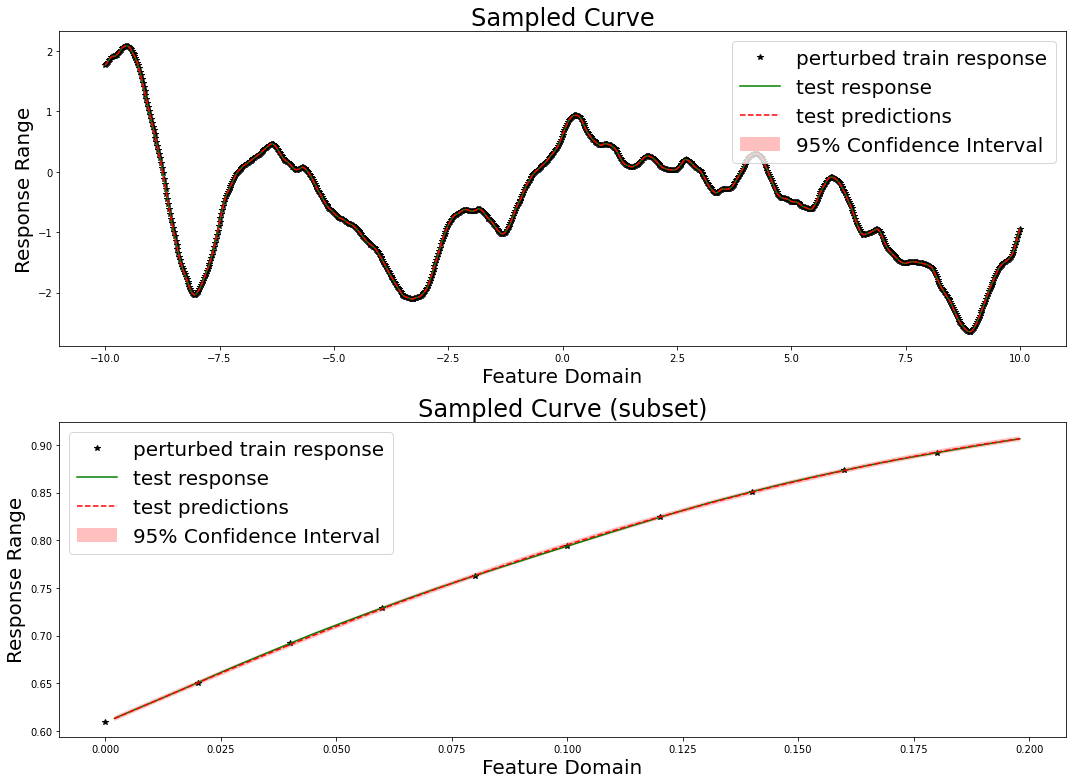
We here evaluate our prediction performance in terms of RMSE, mean diagonal posterior variance, the mean 95% confidence interval size, and the coverage, which ideally should be near 95%.

[20]:

from MuyGPyS.optimize.objective import mse_fn

confidence_intervals = np.sqrt(variances) * 1.96
coverage = (
    np.count_nonzero(
        np.abs(test_responses - predictions)
        < confidence_intervals.reshape(test_count, 1)
    )
    / test_count
)
print(f"RMSE: {np.sqrt(mse_fn(predictions, test_responses))}")
print(f"mean diagonal variance: {np.mean(variances)}")
print(f"mean confidence interval size: {np.mean(confidence_intervals * 2)}")
print(f"coverage: {coverage}")

RMSE: 0.0013556922430336428
mean diagonal variance: 1.7126198738463391e-06
mean confidence interval size: 0.00512938281789808
coverage: 0.9381111111111111

Again, if you do not need to reuse your tensors, you can run the more compact workflow:

[21]:

# # make the indices
# test_count, _ = test_features.shape
# indices = np.arange(test_count)
# nn_indices, _ = nbrs_lookup.get_nns(test_features)

# predictions, variance = muygps.regress_from_indices(
#     indices,
#     nn_indices,
#     test_features,
#     train_features,
#     train_responses,
#     variance_mode="diagonal",
#     apply_sigma_sq=True,
# )

These regression examples return predictions (posterior means) and variances for each element of the test dataset. These variances are in the form of diagonal and independent variances that encode the uncertaintainty of the model’s predictions at each test point. To scale the predictions, they should be multiplied by the trained sigma_sq scaling parameters, of which there will be one scalar associated with each dimension of the response. The kwarg apply_sigma_sq=True indicates that this scaling will be performed automatically. This is the default behavior, but will be skipped if sigma_sq == "unlearned".

For a univariate resonse whose variance is obtained with apply_sigma_sq=False, the scaled predicted variance is equivalent to multiplying the predicted variances by muygps.sigma_sq().

[22]:

# predictions, variances = muygps.regress_from_indices(
#     indices,
#     nn_indices,
#     test_features,
#     train_features,
#     train_responses,
#     variance_mode="diagonal",
#     apply_sigma_sq=False,
# )
# scaled_variance = muygps.sigma_sq() * variances

We can also plot our responses and evaluate their performance. We plot below the predicted and true curves, as well as the 95% confidence interval. We plot a smaller subset of the data in the lower curve in order to better scrutinize the 95% confidence interval.

[23]:

fig, axes = plt.subplots(2, 1, figsize=(15, 11))

axes[0].set_title("Sampled Curve", fontsize=24)
axes[0].set_xlabel("Feature Domain", fontsize=20)
axes[0].set_ylabel("Response Range", fontsize=20)
axes[0].plot(train_features, train_responses, "k*", label="perturbed train response")
axes[0].plot(test_features, test_responses, "g-", label="test response")
axes[0].plot(test_features, predictions, "r--", label="test predictions")
axes[0].fill_between(
    test_features[:, 0],
    (predictions[:, 0] - confidence_intervals),
    (predictions[:, 0] + confidence_intervals),
    facecolor="red",
    alpha=0.25,
    label="95% Confidence Interval",
)
axes[0].legend(fontsize=20)

axes[1].set_title("Sampled Curve (subset)", fontsize=24)
axes[1].set_xlabel("Feature Domain", fontsize=20)
axes[1].set_ylabel("Response Range", fontsize=20)
axes[1].plot(
    train_features[mid:mid + vis_subset_size],
    train_responses[mid:mid + vis_subset_size],
    "k*", label="perturbed train response"
)
axes[1].plot(
    test_features[mid * (train_step - 1):mid * (train_step - 1) + (vis_subset_size * (train_step - 1))],
    test_responses[mid * (train_step - 1):mid * (train_step - 1) + (vis_subset_size * (train_step - 1))],
    "g-", label="test response"
)
axes[1].plot(
    test_features[mid * (train_step - 1):mid * (train_step - 1) + (vis_subset_size * (train_step - 1))],
    predictions[mid * (train_step - 1):mid * (train_step - 1) + (vis_subset_size * (train_step - 1))],
    "r--", label="test predictions")
axes[1].fill_between(
    test_features[mid * (train_step - 1):mid * (train_step - 1) + (vis_subset_size * (train_step - 1))][:, 0],
    (predictions[:, 0] - confidence_intervals)[mid * (train_step - 1):mid * (train_step - 1) + (vis_subset_size * (train_step - 1))],
    (predictions[:, 0] + confidence_intervals)[mid * (train_step - 1):mid * (train_step - 1) + (vis_subset_size * (train_step - 1))],
    facecolor="red",
    alpha=0.25,
    label="95% Confidence Interval",
)
axes[1].legend(fontsize=20)

plt.tight_layout()

plt.show()

../_images/examples_univariate_regression_tutorial_48_0.png