Copyright 2021-2024 Lawrence Livermore National Security, LLC and other MuyGPyS Project Developers. See the top-level COPYRIGHT file for details.
SPDX-License-Identifier: MIT
Anisotropic Metric Tutorial
This notebook walks through a simple anisotropic regression workflow and illustrates anisotropic features of MuyGPyS.
[2]:
import numpy as np

from MuyGPyS._test.sampler import UnivariateSampler2D, print_results
from MuyGPyS.gp import MuyGPS
from MuyGPyS.gp.deformation import Anisotropy, Isotropy, l2
from MuyGPyS.gp.hyperparameter import AnalyticScale, Parameter, VectorParameter
from MuyGPyS.gp.kernels import Matern
from MuyGPyS.gp.noise import HomoscedasticNoise
from MuyGPyS.neighbors import NN_Wrapper
from MuyGPyS.optimize import Bayes_optimize
from MuyGPyS.optimize.batch import sample_batch
from MuyGPyS.optimize.loss import lool_fn
We will set a random seed here for consistency when building docs. In practice we would not fix a seed.
[3]:
np.random.seed(0)
Sampling a 2D Surface from a Conventional GP
This notebook will use a simple two-dimensional curve sampled from a conventional Gaussian process. We will specify the domain as a simple grid on a one-dimensional surface and divide the observations näively into train and test data.
Feel free to download the source notebook and experiment with different parameters.
First we specify the data size and the proportion of the train/test split.
[4]:
points_per_dim = 60
train_ratio = 0.05
We will assume that the true data is produced with no noise, so we specify a very small noise prior for numerical stability. This is an idealized experiment with effectively no instrument error.
[5]:
nugget_noise = HomoscedasticNoise(1e-14)
We will perturb our simulated observations (the training data) with some i.i.d Gaussian measurement noise.
[6]:
measurement_noise = HomoscedasticNoise(1e-7)
Finally, we will specify a Matérn kernel with hyperparameters. smoothness determines how differentiable the GP prior is. The larger smoothness grows, the smoother sampled functions will become.
[7]:
sim_smoothness = Parameter(1.5)
We will use an anisotropic deformation, where displacement along the dimensions are weighted differently. Each dimension has a corresponding length_scale parameter.
[8]:
sim_length_scale0 = Parameter(0.1)
sim_length_scale1 = Parameter(0.5)
We use all of these parameters to define a Matérn kernel GP and a sampler for convenience. The UnivariateSampler2D class is a convenience class for this tutorial, and is not a part of the library. We will use an anisotropic deformation to ensure that we sample data from the appropriate distribution.
[9]:
sampler = UnivariateSampler2D(
    points_per_dim=points_per_dim,
    train_ratio=train_ratio,
    kernel=Matern(
        smoothness=sim_smoothness,
        deformation=Anisotropy(
            l2,
            length_scale=VectorParameter(
                sim_length_scale0,
                sim_length_scale1,
            ),
        ),
    ),
    noise=nugget_noise,
    measurement_noise=measurement_noise,
)
Finally, we will sample a curve from this GP prior and visualize it. Note that we perturb the train responses (the values that our model will actual receive) with Gaussian measurement noise. Further note that this is not especially fast, as sampling from a conventional Gaussian process requires computing the Cholesky decomposition of a (data_count, data_count) matrix.
[10]:
train_features, test_features = sampler.features()
[11]:
train_responses, test_responses = sampler.sample()
[12]:
sampler.plot_sample()
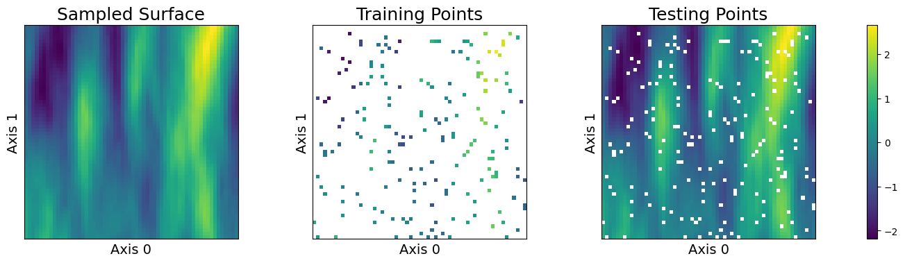
We can observe that our choice of anisotropy has caused the globular Gaussian features in the sampled surface to “smear” in the direction of the more heavily weighted axis.
Training an Anisotropic Model
We will not belabor the details covered in the Univariate Regression Tutorial. We must similarly construct a nearest neighbors index and sample a training batch in order to optimize a model.
⚠️ For now, we use isotropic nearest neighbors as we do not have a guess as to the anisotropic scaling. Future versions of the library will use learned anisotropy to modify neighborhood structure during optimization. ⚠️
[13]:
nn_count = 30
nbrs_lookup = NN_Wrapper(train_features, nn_count, nn_method="exact", algorithm="ball_tree")
batch_count = sampler.train_count
batch_indices, batch_nn_indices = sample_batch(
    nbrs_lookup, batch_count, sampler.train_count
)
We construct a MuyGPs object with a Matérn kernel. For simplicity, we will fix smoothness and attempt to optimize the two length_scale parameters.
[14]:
muygps_anisotropic = MuyGPS(
    kernel=Matern(
        smoothness=sim_smoothness,
        deformation=Anisotropy(
            l2,
            length_scale=VectorParameter(
                Parameter("log_sample", (0.01, 1.0)),
                Parameter("log_sample", (0.01, 1.0)),
            ),
        ),
    ),
    noise=measurement_noise,
    scale=AnalyticScale(),
)
We will also create and optimze an isotropic model for comparison.
[15]:
muygps_isotropic = MuyGPS(
    kernel=Matern(
        smoothness=sim_smoothness,
        deformation=Isotropy(
            l2,
            length_scale=Parameter("log_sample", (0.01, 1.0)),
        ),
    ),
    noise=measurement_noise,
)
We build our difference tensors as usual and use Bayesian optimization. Note that there is a difference between the crosswise and pairwise tensors that we create here, versus those we create for an isotropic kernel. Anisotropic models create difference tensors rather than distance tensors, which have an extra dimension recording the feature dimension-wise comparisons (in this case, differences) between the items being compared. This is an important distinction, as anisotropic models need to record feature-dimension-wise comparisons to be scaled by trainable parameters, whereas isotropic models do not and collapse differences directory into distances.
[16]:
(
    batch_crosswise_diffs,
    batch_pairwise_diffs,
    batch_targets,
    batch_nn_targets,
) = muygps_anisotropic.make_train_tensors(
    batch_indices,
    batch_nn_indices,
    train_features,
    train_responses,
)
Keyword arguments for the optimization:
[17]:
opt_kwargs = {
    "loss_fn": lool_fn,
    "verbose": True,
    "random_state": 1,
    "init_points": 5,
    "n_iter": 30,
    "allow_duplicate_points": True,
}
[18]:
muygps_anisotropic = Bayes_optimize(
    muygps_anisotropic,
    batch_targets,
    batch_nn_targets,
    batch_crosswise_diffs,
    batch_pairwise_diffs,
    **opt_kwargs,
)
parameters to be optimized: ['length_scale0', 'length_scale1']
bounds: [[0.01 1.  ]
 [0.01 1.  ]]
initial x0: [0.07655293 0.30564372]
|   iter    |  target   | length... | length... |
-------------------------------------------------
| 1         | 574.83338 | 0.0765529 | 0.3056437 |
| 2         | 440.21684 | 0.4228517 | 0.7231212 |
| 3         | 301.56409 | 0.0101132 | 0.3093092 |
| 4         | 251.94565 | 0.1552883 | 0.1014152 |
| 5         | 458.89835 | 0.1943976 | 0.3521051 |
| 6         | 389.45339 | 0.4027997 | 0.5434285 |
| 7         | 239.08267 | 0.6737628 | 0.4605208 |
| 8         | 424.18428 | 0.4503475 | 0.7163531 |
| 9         | 553.28388 | 0.1019755 | 0.3088795 |
| 10        | 573.19170 | 0.0800375 | 0.3060548 |
| 11        | 573.71590 | 0.1179995 | 0.7801772 |
| 12        | 579.62072 | 0.1840045 | 0.7730065 |
| 13        | 581.24279 | 0.1606255 | 0.8432544 |
| 14        | 562.17347 | 0.2458237 | 0.8361934 |
| 15        | 491.44103 | 0.0672756 | 0.8613874 |
| 16        | 578.29506 | 0.2101782 | 0.9231864 |
| 17        | 549.92797 | 0.3002584 | 0.9281173 |
| 18        | 586.60160 | 0.1388571 | 0.6850706 |
| 19        | 490.70978 | 0.0491339 | 0.6928365 |
| 20        | 549.79030 | 0.2250734 | 0.6799292 |
| 21        | 576.63747 | 0.1578857 | 0.5945186 |
| 22        | 564.80882 | 0.1507120 | 1.0       |
| 23        | 580.01112 | 0.0760850 | 0.5421669 |
| 24        | 563.28524 | 0.1532621 | 0.4984400 |
| 25        | 574.10561 | 0.2453701 | 1.0       |
| 26        | 518.54556 | 0.3959557 | 1.0       |
| 27        | 585.52893 | 0.0696432 | 0.4556013 |
| 28        | 331.35809 | 0.01      | 0.5047835 |
| 29        | 577.06821 | 0.1140036 | 0.4145796 |
| 30        | 582.43687 | 0.0928413 | 0.6099512 |
| 31        | 358.85291 | 0.0376719 | 1.0       |
| 32        | 447.33495 | 0.5628038 | 1.0       |
| 33        | 581.26564 | 0.1610530 | 0.8436895 |
| 34        | 586.60474 | 0.1387601 | 0.6851618 |
| 35        | -555.4362 | 1.0       | 0.01      |
| 36        | 321.45269 | 1.0       | 1.0       |
=================================================
[19]:
print(f"BayesianOptimization finds an optimimal pair of length scales: {muygps_anisotropic.kernel.deformation.length_scale()}")
BayesianOptimization finds an optimimal pair of length scales: [0.13876015 0.68516186]
Note here that these returned length scale values might be a little different than what we used to sample the surface. This can be due to a few factors: 1. optimizer might not have run enough iterations to converge, or 2. there is some mutual unidentifiability between the length scale parameters and the variance scale parameter.
However, length_scale0 < length_scale1 as expected.
We also optimize the isotropic benchmark. Notice that we need to construct new distance tensors for the isotropic model.
[20]:
(
    batch_crosswise_dists,
    batch_pairwise_dists,
    _,
    _,
) = muygps_isotropic.make_train_tensors(
    batch_indices,
    batch_nn_indices,
    train_features,
    train_responses,
)
[21]:
muygps_isotropic = Bayes_optimize(
    muygps_isotropic,
    batch_targets,
    batch_nn_targets,
    batch_crosswise_dists,
    batch_pairwise_dists,
    **opt_kwargs,
)
parameters to be optimized: ['length_scale']
bounds: [[0.01 1.  ]]
initial x0: [0.83917142]
|   iter    |  target   | length... |
-------------------------------------
| 1         | -33432.37 | 0.8391714 |
| 2         | -3484.032 | 0.4228517 |
| 3         | -21027.54 | 0.7231212 |
| 4         | -151.5398 | 0.0101132 |
| 5         | -903.5748 | 0.3093092 |
| 6         | 324.47361 | 0.1552883 |
| 7         | 249.64357 | 0.0810921 |
| 8         | 335.25399 | 0.1460524 |
| 9         | 335.26767 | 0.1460362 |
| 10        | 71.800309 | 0.2194212 |
| 11        | 330.64599 | 0.1167226 |
| 12        | 340.13530 | 0.1310462 |
| 13        | 340.26578 | 0.1318735 |
| 14        | 340.34770 | 0.1326687 |
| 15        | 340.38871 | 0.1335571 |
| 16        | 334.99671 | 0.1211132 |
| 17        | 340.18714 | 0.1362445 |
| 18        | 340.22616 | 0.1359973 |
| 19        | 340.27916 | 0.1356084 |
| 20        | 289.66935 | 0.1718813 |
| 21        | 339.49010 | 0.1286277 |
| 22        | 339.98942 | 0.1372330 |
| 23        | 339.44388 | 0.1284965 |
| 24        | 339.78544 | 0.1380161 |
| 25        | 339.55813 | 0.1288271 |
| 26        | 339.74443 | 0.1381565 |
| 27        | 339.66966 | 0.1291724 |
| 28        | 339.75201 | 0.1381309 |
| 29        | 339.76162 | 0.1294778 |
| 30        | 339.78164 | 0.1380293 |
| 31        | 339.83539 | 0.1297393 |
| 32        | 339.82320 | 0.1378825 |
| 33        | 339.89839 | 0.1299766 |
| 34        | 339.87224 | 0.1377022 |
| 35        | 339.95258 | 0.1301933 |
| 36        | 339.92684 | 0.1374910 |
=====================================
[22]:
print(f"BayesianOptimization finds that the optimimal isotropic length scale is {muygps_isotropic.kernel.deformation.length_scale()}")
BayesianOptimization finds that the optimimal isotropic length scale is 0.13355719498402782
We see here that when fixed to an isotropic length scale, Bayesian optimization tends to favor the smallest true length scale. We’ll see how this affects modeling, prediction, and uncertainty quanlity below.
We separately optimize the scale variance scale parameter for each model.
[23]:
muygps_anisotropic = muygps_anisotropic.optimize_scale(
    batch_pairwise_diffs, batch_nn_targets
)
muygps_isotropic = muygps_isotropic.optimize_scale(
    batch_pairwise_diffs, batch_nn_targets
)
Inference
As in the Univariate Regression Tutorial, we must realize difference tensors formed from the testing data and apply them to form Gaussian process predictions for our problem.
[24]:
test_count, _ = test_features.shape
indices = np.arange(test_count)
test_nn_indices, _ = nbrs_lookup.get_nns(test_features)
(
    test_crosswise_diffs,
    test_pairwise_diffs,
    test_nn_targets,
) = muygps_anisotropic.make_predict_tensors(
    indices,
    test_nn_indices,
    test_features,
    train_features,
    train_responses,
)
(
    test_crosswise_dists,
    test_pairwise_dists,
    _,
) = muygps_isotropic.make_predict_tensors(
    indices,
    test_nn_indices,
    test_features,
    train_features,
    train_responses,
)
As in the Univariate Regression Tutorial we will evaluate the prediction performance of our models in terms of RMSE, mean diagonal posterior variance, the mean 95% confidence interval size, and the coverage, which ideally should be near 95%.
[25]:
Kcross_anisotropic = muygps_anisotropic.kernel(test_crosswise_diffs)
Kin_anisotropic = muygps_anisotropic.kernel(test_pairwise_diffs)

predictions_anisotropic = muygps_anisotropic.posterior_mean(
    Kin_anisotropic, Kcross_anisotropic, test_nn_targets
)
variances_anisotropic = muygps_anisotropic.posterior_variance(
    Kin_anisotropic, Kcross_anisotropic
)
confidence_intervals_anisotropic = np.sqrt(variances_anisotropic) * 1.96
coverage_anisotropic = (
    np.count_nonzero(
        np.abs(test_responses - predictions_anisotropic) < confidence_intervals_anisotropic
    ) / test_count
)
We also evaluate the isotropic model
[26]:
Kcross_isotropic = muygps_isotropic.kernel(test_crosswise_dists)
Kin_isotropic = muygps_isotropic.kernel(test_pairwise_dists)

predictions_isotropic = muygps_isotropic.posterior_mean(Kin_isotropic, Kcross_isotropic, test_nn_targets)
variances_isotropic = muygps_isotropic.posterior_variance(Kin_isotropic, Kcross_isotropic)

confidence_intervals_isotropic = np.sqrt(variances_isotropic) * 1.96
coverage_isotropic = (
    np.count_nonzero(
        np.abs(test_responses - predictions_isotropic) < confidence_intervals_isotropic
    ) / test_count
)
Results comparison
A comparison of our trained models reveals that the anisotropic kernel gets close to the true (0.1, 0.5) length scale, whereas the isotropic model has to learn a single parameter that has to split the difference somehow. This results in both a higher RMSE and larger confidence intervals in order to achieve similar coverage.
[27]:
print_results(
    test_responses,
    ("anisotropic", muygps_anisotropic, predictions_anisotropic, variances_anisotropic, confidence_intervals_anisotropic, coverage_anisotropic),
    ("isotropic", muygps_isotropic, predictions_isotropic, variances_isotropic, confidence_intervals_isotropic, coverage_isotropic),
)
[27]:
| name | smoothness | length scale | noise variance | variance scale | rmse | mean variance | mean confidence interval | coverage |
|---|---|---|---|---|---|---|---|---|
| anisotropic | 1.500000 | [0.13876015 0.68516186] | 0.000000 | 2.036444 | 0.139218 | 0.020339 | 0.242004 | 0.942690 |
| isotropic | 1.500000 | 0.133557 | 0.000000 | 1.000000 | 0.285544 | 0.083572 | 0.514294 | 0.952047 |
This dataset is low-dimensional so we can plot our predictions and visually evaluate their performance. We plot below the expected (true) surface, and the surface that our model predicts. Note that they are visually similar and major trends are captured, although there are some differences.
[28]:
sampler.plot_predictions(("Anisotropic", predictions_anisotropic), ("Isotropic", predictions_isotropic))

As we can see, the anisotropic model learns a surface that is much visually closer to what is expected. In particular, the isotropic surface has blobby circular features as it to be expected, as it is unable to differentiate between distances along the different axes.
We will also investigate more details information about the errors. Below we produce three plots that help us to understand our results. The left plot shows the residual, which is the difference between the true values and our expectations. The middle plot shows the magnitude of the 95% confidence interval. The larger the confidence interval, the less certain the model is of its predictions. Finally, the right plot shows the difference between the 95% confidence interval length and the magnitude of the residual. All of the points larger than zero (in red) are not captured by the confidence interval. Hence, this plot shows our coverage distribution.
[29]:
sampler.plot_errors(
    ("Anisotropic", predictions_anisotropic, confidence_intervals_anisotropic),
    ("Isotropic", predictions_isotropic, confidence_intervals_isotropic),
)

The rightmost columns shows that the anisotropic assumptions both obtains lower residuals, i.e. the posterior means are more accurate. The middle column shows that the the posterior variances (and resulting confidence intervals) are smaller, and therefore the anisotropic model is also more confident in its predictions. Finally, the rightmost plot reveals the uncovered points - all red-scale residuals exceed the confidence interval. Not only does the isotropic model appear to have more uncovered points, they tend to be further outside of the confidence interval than those of the anisotropic model. These results demonstrate the importance of correct model assumptions, both on predictions and uncertainty quantification.