SPDX-License-Identifier: MIT

Fast Posterior Mean Tutorial

This notebook walks through the fast posterior mean workflow presented in Fast Gaussian Process Posterior Mean Prediction via Local Cross Validation and Precomputation (Dunton et. al 2022) and explains the relevant components of MuyGPyS.

The cell below uses the same code as that found in univariate_regression_tutorial.ipynb. This includes generating the synthetic data from a GP and training two MuyGPs models to fit the data using Bayesian optimization.

[2]:

import matplotlib.pyplot as plt
import numpy as np
import pandas as pd
import timeit

from MuyGPyS._test.gp import benchmark_sample, BenchmarkGP
from MuyGPyS._test.sampler import UnivariateSampler, print_fast_results
from MuyGPyS.neighbors import NN_Wrapper
from MuyGPyS.gp import MuyGPS
from MuyGPyS.gp.deformation import Isotropy, l2
from MuyGPyS.gp.hyperparameter import AnalyticScale, Parameter
from MuyGPyS.gp.kernels import Matern
from MuyGPyS.gp.noise import HomoscedasticNoise
from MuyGPyS.gp.tensors import (
    crosswise_tensor,
    fast_nn_update,
    pairwise_tensor,
    make_fast_predict_tensors,
    make_predict_tensors,
)

We will assume that we have already optimized the a MuyGPs model following the Univariate Regression Tutorial.

[3]:

kernel = Matern(
    smoothness=Parameter(2.0),
    deformation=Isotropy(
        l2,
        length_scale=Parameter(0.05),
    ),
)

We will use that kernel to simulate a curve and then compare the prediction times for both the conventional regression and the fast kernel regression method.

[4]:

np.random.seed(0)
measurement_noise = 1e-4
sampler = UnivariateSampler(
    data_count=3000,
    train_ratio=0.1,
    kernel=kernel,
    noise=HomoscedasticNoise(1e-14),
    measurement_noise=HomoscedasticNoise(measurement_noise),
)
train_features, test_features = sampler.features()
test_count, _ = test_features.shape
train_count, _ = train_features.shape

[5]:

train_responses, test_responses = sampler.sample()

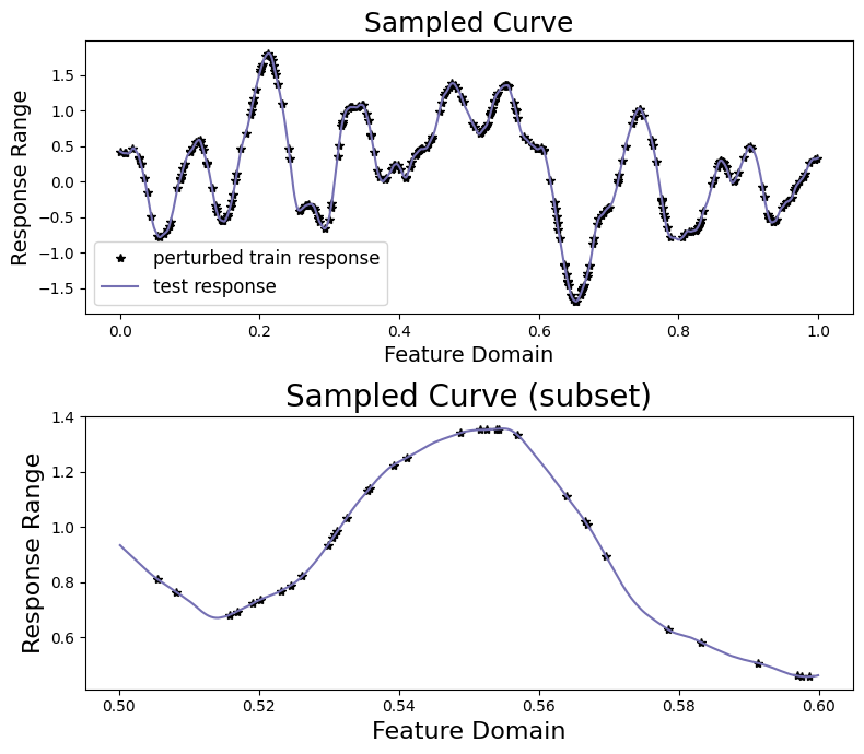
We’ll visualize the results.

[6]:

sampler.plot_sample()

../_images/examples_fast_regression_tutorial_11_0.png

We then prepare a MuyGPS object and a nearest neighbors index. We could use a single MuyGPS object, but in this case we create a second one for the fast regression because a larger noise prior helps to stabilize the computations.

[7]:

nbrs_lookup = NN_Wrapper(train_features, nn_count=10, nn_method="exact",algorithm="ball_tree")
muygps = MuyGPS(
    kernel=kernel,
    noise=HomoscedasticNoise(1e-4),
    scale=AnalyticScale(),
)
muygps_fast = MuyGPS(
    kernel=kernel,
    noise=HomoscedasticNoise(1e-1),
    scale=AnalyticScale(),
)

Benchmarking Fast Prediction

With set (or learned) hyperparameters, we are able to use the muygps object for fast prediction capability.

See below a fast posterior mean workflow, using the data structures built up in this example. This workflow uses the compact tensor-making function make_fast_predict_tensors() to succinctly create tensors defining the pairwise_diffs among each nearest neighbor and the train_nn_targets_fast or responses of the nearest neighbors in each set. We then create theK covariance tensor and form the precomputed coefficients matrix. We then pass the precomputed coefficients matrix, the nn_indices matrix of neighborhood indices, and the closest neighbor of each test point to MuyGPS.fast_posterior_mean() in order to obtain our predictions.

First we obtain the indices of the nearest neighbors of all of the training datapoints.

[8]:

train_nn_indices, _ = nbrs_lookup.get_nns(train_features)

We then update these neighborhoods with the index of the corresponding training point so that each neighborhood contains the query point.

[9]:

train_nn_indices_fast = fast_nn_update(train_nn_indices)

We then compute the pairwise difference tensor and target matrix and use them to construct the corresponding kernel tensor and the precomputed target matrix to be used in the fast kernel regression.

[10]:

pairwise_diffs_fast, nn_targets_fast = make_fast_predict_tensors(
    train_nn_indices_fast,
    train_features,
    train_responses,
)
K_fast = muygps_fast.kernel(pairwise_diffs_fast)
precomputed_coefficients_matrix = muygps_fast.fast_coefficients(K_fast, nn_targets_fast)

The steps so far have involved only the training data, and can be precomputed before encountering the test data. We now find the closest training point to each test point and return the corresponding enriched training points.

[11]:

test_indices = np.arange(test_count)
test_nn_indices, _ = nbrs_lookup.get_nns(test_features)
closest_neighbor = test_nn_indices[:, 0]
closest_set = train_nn_indices_fast[closest_neighbor, :]

We use these indices to make the crosswise difference tensor, similar to usual prediction.

[12]:

crosswise_diffs_fast = crosswise_tensor(test_features, train_features, test_indices, closest_set)

Finally, we compute the crosscovariance and perform fast prediction.

[13]:

Kcross_fast = muygps_fast.kernel(crosswise_diffs_fast)
predictions_fast = muygps_fast.fast_posterior_mean(
    Kcross_fast,
    precomputed_coefficients_matrix[closest_neighbor,:,:])

Comparison with Conventional Prediction

With set (or learned) hyperparameters, we are able to use the muygps object to predict the response of test data. Several workflows are supported.

See below a simple posterior mean workflow, using the data structures built up in this example. This is very similar to the prediction workflow found in the univariate regression tutorial.

[14]:

(
    crosswise_diffs,
    pairwise_diffs,
    nn_targets,
) = make_predict_tensors(
    np.arange(test_count),
    test_nn_indices,
    test_features,
    train_features,
    train_responses,
)
Kcross = muygps.kernel(crosswise_diffs)
K = muygps.kernel(pairwise_diffs)
predictions = muygps.posterior_mean(
    K, Kcross, nn_targets
)
variances = muygps.posterior_variance(K, Kcross)
confidence_intervals = np.sqrt(variances) * 1.96
coverage = np.count_nonzero(np.abs(test_responses - predictions) < confidence_intervals) / test_count

We compare our two methods in terms of time-to-solution and RMSE. In the conventional workflow we compute the sum of the time it takes to: - identify the nearest neighbors of the test features, - form the relevant kernel tensors, and - solve the posterior means.

In the fast posterior mean case, we compute the sum of the time it takes to: - identify the nearest neighbor of each test point, - lookup coefficients in the precomputed coefficient matrix, and - perform the dot product to form posterior means.

Note that the fast kernel regression method does not compute a variance, and so its posterior variance, confidence intervals, and coverage are nil.

[15]:

def timing_posterior_mean():
    test_nn_indices, _ = nbrs_lookup.get_nns(test_features)
    (
        crosswise_diffs,
        pairwise_diffs,
        nn_targets,
    ) = make_predict_tensors(
        test_indices,
        test_nn_indices,
        test_features,
        train_features,
        train_responses,
    )
    Kcross = muygps.kernel(crosswise_diffs)
    K = muygps.kernel(pairwise_diffs)
    predictions = muygps.posterior_mean(
        K, Kcross, nn_targets
    )

def timing_fast_posterior_mean():
    test_nn_indices_fast, _ = nbrs_lookup.get_nns(test_features)
    closest_neighbor = test_nn_indices_fast[:, 0]
    closest_set = train_nn_indices_fast[closest_neighbor, :].astype(int)
    crosswise_diffs = crosswise_tensor(
        test_features,
        train_features,
        test_indices,
        closest_set,
    )
    Kcross = muygps_fast.kernel(crosswise_diffs)
    predictsion_fast = muygps_fast.fast_posterior_mean(
        Kcross,
        precomputed_coefficients_matrix[closest_neighbor,:,:])

[16]:

time_conv = %timeit -o timing_posterior_mean()
time_fast = %timeit -o timing_fast_posterior_mean()

186 ms ± 383 µs per loop (mean ± std. dev. of 7 runs, 10 loops each)
20.6 ms ± 66.9 µs per loop (mean ± std. dev. of 7 runs, 10 loops each)

[17]:

nil_vec = np.zeros(test_count)
print_fast_results(
    test_responses,
    ("conventional", time_conv, muygps, predictions),
    ("fast", time_fast, muygps_fast, predictions_fast),
)

[17]:

name	rmse	timing results	noise variance
conventional	0.007781	186 ms ± 383 µs per loop (mean ± std. dev. of 7 runs, 10 loops each)	0.000100
fast	0.086229	20.6 ms ± 66.9 µs per loop (mean ± std. dev. of 7 runs, 10 loops each)	0.100000

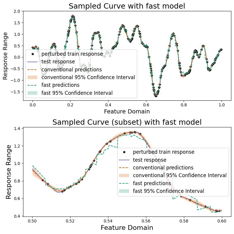
As we can see, we can gain an order of magnitude speed improvement by sacrificing some precision and the posterior variance. We also plot our two methods and compare their results graphically.

[18]:

sampler.plot_results(
    ("conventional", predictions, confidence_intervals),
    ("fast", predictions_fast, np.zeros(test_count)),
)

../_images/examples_fast_regression_tutorial_34_0.png