Copyright 2021-2024 Lawrence Livermore National Security, LLC and other MuyGPyS Project Developers. See the top-level COPYRIGHT file for details.
SPDX-License-Identifier: MIT
Loss Function Tutorial
This notebook illustrates the loss functions available in the MuyGPyS library. These functions are used to formulate the objective function to be optimized while fitting hyperparameters, and so have a large effect on the outcome of training. We will describe each of these loss functions and plot their behaviors to help the user to select the right loss for their problem.
Each function in this notebook is available for import from MuyGPyS.optimize.loss, and is an object of class MuyGPyS.optimize.loss.LossFn. It is possible to define new loss functions by creating a new LossFn object. View its documentation for more details.
We assume throughout a vector of targets \(y\), a prediction (posterior mean) vector \(\mu\), and a posterior variance vector \(\sigma\) for a training batch \(B\) with \(b\) elements.
[2]:
import matplotlib.pyplot as plt
import numpy as np

import cblind as cb
from matplotlib.colors import SymLogNorm, LogNorm
from MuyGPyS.optimize.loss import mse_fn, cross_entropy_fn, lool_fn, pseudo_huber_fn, looph_fn
[3]:
plt.style.use('tableau-colorblind10')
[4]:
mmax = 3.0
mmin = 0.0
residual_count = 100
ys = np.zeros(residual_count)
residuals = np.linspace(mmin, mmax, residual_count)
smax = 3.0
smin = 1e-1
variance_count = 100
variances = np.linspace(smin, smax, variance_count)
unitary_scale=np.ones(1)
Variance-free Loss Functions
MuyGPyS features several loss functions that depend only upon the targets \(y\) and posterior mean predictions \(\hat{\mu}\) of your training batch. These loss functions are situationally useful, although they leave the fitting of variance parameters entirely up to the separate, scale optimization functions and might not be sensitive to certain variance parameters. As they do not require evaluating the posterior variance \(\hat{\Sigma}\) or optimizing the variance scale parameter
\(\sigma^2\), these loss functions are generally more efficient to use in practice.
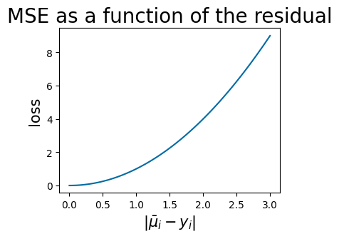
Mean Squared Error (mse_fn)
The mean squared error (MSE) or \(\ell_2\) loss is a classic loss function that computes
\begin{equation*} \ell_\textrm{MSE}(\bar{\mu}, y) = \frac{1}{b} \sum_{i \in B} (\bar{\mu}_i - y_i)^2. \end{equation*}
The following plot illustrates the MSE as a function of the residual.
[5]:
fig, ax = plt.subplots(1, 1, figsize=(4,3))
ax.set_title("MSE as a function of the residual", fontsize=20)
ax.set_ylabel("loss", fontsize=15)
ax.set_xlabel(r"$\vert \bar{\mu}_i - y_i \vert$", fontsize=15)
mses = np.array([mse_fn(ys[i], residuals[i]) for i in range(residual_count)])
ax.plot(residuals, mses)
plt.show()
Cross Entropy Loss (cross_entropy_fn)
The cross entropy loss is a classic classification loss often used in the fitting of neural networks. For targets in \(\{0, 1\}\), the library first transforms the predictions to be row-stochastic and then computes
\begin{equation*} \ell_\textrm{cross-entropy}(\bar{\mu}, y) = \sum_{i \in B} y_i \log(\bar{\mu}_i) - (1 - y_i) \log(1 - \bar{\mu}_i) \end{equation*}
⚠️ This section is under construction. ⚠️
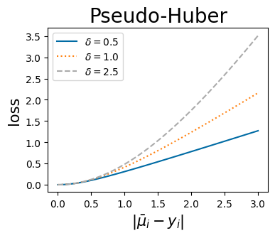
Pseudo-Huber Loss (pseudo_huber_fn)
The pseudo-Huber loss is a smooth approximation to the Huber loss, which is approximately quadratic (\(\ell_2\) loss) for small residuals and approximately linear (\(\ell_1\) loss) for large residuals. This means that the pseudo-Huber loss is less sensitive to large outliers, which might otherwise force the optimizer to overcompensate in undesirable ways. The pseudo-Huber loss computes
\begin{equation*} \ell_\textrm{Pseudo-Huber} \left ( \bar{\mu}, y \mid \delta \right ) = \sum_{i=1}^b \delta^2 \left ( \sqrt{1 + \left ( \frac{\bar{\mu}_i - y_i}{\delta} \right )^2} - 1 \right ), \end{equation*}
where \(\delta\) is a parameter that indicates the scale of the boundary between the quadratic and linear parts of the function. The pseudo_huber_fn accepts this parameter as the boundary_scale keyword argument. Note that the scale of \(\delta\) depends on the units of \(y\) and \(\hat{\mu}\). The following plots show the behavior of the pseudo-Huber loss for a few values of \(\delta\).
[6]:
boundary_scales = [0.5, 1.0, 2.5]
phs = np.array([
    [pseudo_huber_fn(ys[i], residuals[i], boundary_scale=bs) for i in range(residual_count)]
    for bs in boundary_scales
])
fig, ax = plt.subplots(1, 1, figsize=(4, 3))
# for i, ax in enumerate(axes):
ax.set_title(f"Pseudo-Huber", fontsize=20)
ax.set_ylabel("loss", fontsize=15)
ax.set_xlabel(r"$\vert \bar{\mu}_i - y_i \vert$", fontsize=15)
ax.plot(residuals, phs[0, :], linestyle="solid", label=f"$\delta = {boundary_scales[0]}$")
ax.plot(residuals, phs[1, :], linestyle="dotted", label=f"$\delta = {boundary_scales[1]}$")
ax.plot(residuals, phs[2, :], linestyle="dashed", label=f"$\delta = {boundary_scales[2]}$")
ax.legend()
plt.show()
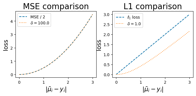
Coincidence of pseudo-Huber and MSE for relatively small residuals
For large boundary scales relative the residual magnitude, the pseudo-Huber function converges to 1/2 of the \(\ell_2\) loss or mean squared error, as show by the next figure. This convergence is relative to the scale of the residual, and so the value of the boundary scale is informed by the data distribution and requires the user to reason about the breakpoint where residuals are likely to be unreasonably large. Similarly, when \(\delta=1\) the pseudo-huber loss is parallel to \(\ell_1\) loss for larger residuals.
[7]:
def l1_fn(
    predictions: np.ndarray,
    targets: np.ndarray,
) -> float:
    return np.sum(np.abs(predictions - targets))

l1s = np.array([l1_fn(ys[i], residuals[i]) for i in range(residual_count)])
[8]:
big_boundary_scale = 100.0
sml_boundary_scale = 1.0
big_ph = np.array([
    pseudo_huber_fn(ys[i], residuals[i], boundary_scale=big_boundary_scale)
    for i in range(residual_count)
])
sml_ph = np.array([
    pseudo_huber_fn(ys[i], residuals[i], boundary_scale=sml_boundary_scale)
    for i in range(residual_count)
])
fig, axes = plt.subplots(1, 2, figsize=(8,3))
axes[0].set_title("MSE comparison", fontsize=20)
axes[0].set_ylabel("loss", fontsize=15)
axes[0].set_xlabel(r"$\vert \bar{\mu}_i - y_i \vert $", fontsize=15)
axes[0].plot(residuals, mses / 2, linestyle="dashed", label=f"MSE / 2")
axes[0].plot(residuals, big_ph, linestyle="dotted", label=f"$\delta = {big_boundary_scale}$")
axes[0].legend()

axes[1].set_title("L1 comparison", fontsize=20)
axes[1].set_ylabel("loss", fontsize=15)
axes[1].set_xlabel(r"$\vert \bar{\mu}_i - y_i \vert$", fontsize=15)
axes[1].plot(residuals, l1s, linestyle="dashed", label="$\ell_1$ loss")
axes[1].plot(residuals, sml_ph, linestyle="dotted", label=f"$\delta = {sml_boundary_scale}$")
axes[1].legend()
plt.show()
Variance-Sensitive Loss Functions
MuyGPyS also includes loss functions that explicitly depend upon the posterior variances \(\bar{\Sigma}\), which is a diagonal matrix for a univariate MuyGPs model. These loss functions penalize large variances, and so tend to be more sensitive to variance parameters. This comes at increasing the cost of the linear algebra involved in each evaluation of the objective function by a constant factor. This causes an overall increase in compute time per optimization loop, but that is often a
worthwhile trade for sensitivity in practice.
\(\bar{\Sigma}\) involves multiplying the unscaled MuyGPS variance by the \(\sigma^2\) variance scaling parameter, which at present must by optimized during each evaluation of the objective function.
Leave-One-Out Loss (lool_fn)
The leave-one-out-loss or lool scales and regularizes the MSE to make the loss more sensitive to parameters that primarily act on the variance. lool computes
\begin{equation*} \ell_\textrm{lool}(\bar{\mu}, y, \bar{\Sigma}) = \sum_{i \in B} \frac{(\bar{\mu}_i - y_i)^2}{\bar{\Sigma}_{ii}} + \log \bar{\Sigma}_{ii}. \end{equation*}
The next plot illustrates the loss as a function of both the residual and of \(\sigma^2\).
[9]:
lools = np.array([
    [
        lool_fn(
            ys[i],
            residuals[i],
            variances[variance_count - 1 - j],
            unitary_scale,
        )
        for i in range(residual_count)
    ]
    for j in range(variance_count)
])
[10]:
variance_vis_values = [0.5, 1.0, 1.5]
variance_vis_points = list()
var_iter = 0
for i, var in enumerate(variances):
    if var_iter >= len(variance_vis_values):
        break
    if var > variance_vis_values[var_iter]:
        variance_vis_points.append([variance_count - 1 - i, var])
        var_iter += 1
[11]:
residual_vis_values = [0.25, 0.75, 1.25]
residual_vis_points = list()
res_iter = 0
for i, res in enumerate(residuals):
    if res_iter >= len(residual_vis_values):
        break
    if res > residual_vis_values[res_iter]:
        residual_vis_points.append([i, res])
        res_iter += 1
[12]:
style_count = len(variance_vis_values) + len(residual_vis_values)
colors, linestyles = cb.Colorplots().cblind(style_count)
colors = colors[:style_count]
linestyles = linestyles[:style_count]
linestyles = list(reversed(linestyles))
[13]:
fig, axes = plt.subplots(1, 3, figsize=(12, 4))
axes[0].set_title("lool", fontsize=20)
axes[0].set_ylabel(r"$\bar{\Sigma}_{ii}$", fontsize=15)
axes[0].set_xlabel(r"$\vert \bar{\mu}_i - y_i \vert$", fontsize=15)
im = axes[0].imshow(
    lools, extent=[mmin, mmax, smin, smax], norm=SymLogNorm(1e-1), cmap="coolwarm"
)
fig.colorbar(im, ax=axes[0])
axes[0].plot(residuals, variance_count * [variance_vis_points[0][1]], color=colors[0], linestyle=linestyles[0])
axes[0].plot(residuals, variance_count * [variance_vis_points[1][1]], color=colors[1], linestyle=linestyles[1])
axes[0].plot(residuals, variance_count * [variance_vis_points[2][1]], color=colors[2], linestyle=linestyles[2])
axes[0].plot(residual_count * [residual_vis_points[0][1]], variances, color=colors[3], linestyle=linestyles[3])
axes[0].plot(residual_count * [residual_vis_points[1][1]], variances, color=colors[4], linestyle=linestyles[4])
axes[0].plot(residual_count * [residual_vis_points[2][1]], variances, color=colors[5], linestyle=linestyles[5])

axes[1].set_title("lool residual cross-section", fontsize=14)
axes[1].set_ylabel("lool", fontsize=15)
axes[1].set_xlabel(r"$\vert \bar{\mu}_i - y_i \vert $", fontsize=15)
axes[1].plot(
    residuals,
    lools[variance_vis_points[0][0], :],
    color=colors[0],
    linestyle=linestyles[0],
    label=r"$\bar{\Sigma}_{ii} = $" + f"{variance_vis_points[0][1]:.2f}",
)
axes[1].plot(
    residuals,
    lools[variance_vis_points[1][0], :],
    color=colors[1],
    linestyle=linestyles[1],
    label=r"$\bar{\Sigma}_{ii} = $" + f"{variance_vis_points[1][1]:.2f}",
)
axes[1].plot(
    residuals,
    lools[variance_vis_points[2][0], :],
    color=colors[2],
    linestyle=linestyles[2],
    label=r"$\bar{\Sigma}_{ii} = $" + f"{variance_vis_points[2][1]:.2f}",
)
axes[1].legend()

axes[2].set_title("lool, variance cross-section", fontsize=14)
axes[2].set_ylabel("lool", fontsize=15)
axes[2].set_xlabel(r"$\bar{\Sigma}_{ii}$", fontsize=15)
axes[2].plot(
    variances,
    np.flip(lools[:, residual_vis_points[0][0]]),
    color=colors[3],
    linestyle=linestyles[3],
    label=r"$\vert \bar{\mu}_i - y_i \vert = $" + f"{residual_vis_points[0][1]:.2f}",
)
axes[2].plot(
    variances,
    np.flip(lools[:, residual_vis_points[1][0]]),
    color=colors[4],
    linestyle=linestyles[4],
    label=r"$\vert \bar{\mu}_i - y_i \vert = $" + f"{residual_vis_points[1][1]:.2f}",
)
axes[2].plot(
    variances,
    np.flip(lools[:, residual_vis_points[2][0]]),
    color=colors[5],
    linestyle=linestyles[5],
    label=r"$\vert \bar{\mu}_i - y_i \vert = $" + f"{residual_vis_points[2][1]:.2f}",
)
axes[2].legend()

plt.tight_layout()
plt.show()
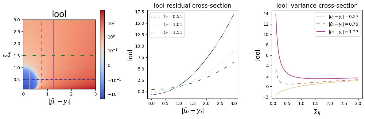
Notice that the cross-section of the lool surface for a fixed \(\sigma\) is quadratic, while the cross section of the lool surface for a fixed residual is logarithmic. For small enough residuals, this curve inverts and assumes negative values for small \(\sigma\).
Leave-One-Out Pseudo-Huber (looph_fn)
The leave-one-out pseudo-Huber loss (looph) is similar in nature to the lool, but is applied to the pseudo-Huber loss instead of MSE. looph computes
\begin{equation*} \ell_\textrm{looph}(\bar{\mu}, y, \bar{\Sigma} \mid \delta) = \sum_{i=1}^b 2\delta^2 \left ( \sqrt{1 + \frac{(\bar{\mu}_i - y_i)^2}{\delta^2 \bar{\Sigma}_{ii}}} - 1 \right ) + \log \bar{\Sigma}_{ii}, \end{equation*}
where again \(\delta\) is the boundary scale.
Note that unlike in the pseudo-Huber, here the boundary scale \(\delta\) is unitless. \(\delta\) specifies how large the residual must be, in multiples of the standard deviation, for the loss to become approximately linear instead of approximately quadratic. As such, there is no need for most applications to set \(\delta\), which the library defaults to 3.0. This implies that only residuals that are larger than 3 standard deviations are treated as outliers.
The next plots illustrate the looph as a function of the residual, \(\sigma\), and \(\delta\) for \(\delta \in \{0.5, 3.0\}\). The plots for the smaller \(\delta\) value illustrates why \(\delta\) should not be small.
[14]:
loo_boundary_scales = np.array([0.5, 3.0])
loophs = np.array([
    [
        [
            looph_fn(
                ys[i],
                residuals[i],
                variances[variance_count - 1 - j],
                unitary_scale,
                boundary_scale=bs
            )
            for i in range(residual_count)
        ]
        for j in range(variance_count)
    ]
    for bs in loo_boundary_scales
])
[15]:
fig, axes = plt.subplots(2, 3, figsize=(14, 4 * len(loo_boundary_scales)))
for i, bs in enumerate(loo_boundary_scales):
    axes[i, 0].set_title(f"looph ($\delta={bs}$)", fontsize=20)
    axes[i, 0].set_ylabel(r"$\bar{\Sigma}_{ii}$", fontsize=15)
    axes[i, 0].set_xlabel(r"$\vert \bar{\mu}_i - y_i \vert$", fontsize=15)
    im = axes[i, 0].imshow(
        loophs[i, :, :], extent=[mmin, mmax, smin, smax], norm=SymLogNorm(1e-1), cmap="coolwarm"
    )
    fig.colorbar(im, ax=axes[i, 0])
    axes[i, 0].plot(residuals, variance_count * [variance_vis_points[0][1]], color=colors[0], linestyle=linestyles[0])
    axes[i, 0].plot(residuals, variance_count * [variance_vis_points[1][1]], color=colors[1], linestyle=linestyles[1])
    axes[i, 0].plot(residuals, variance_count * [variance_vis_points[2][1]], color=colors[2], linestyle=linestyles[2])
    axes[i, 0].plot(residual_count * [residual_vis_points[0][1]], variances, color=colors[3], linestyle=linestyles[3])
    axes[i, 0].plot(residual_count * [residual_vis_points[1][1]], variances, color=colors[4], linestyle=linestyles[4])
    axes[i, 0].plot(residual_count * [residual_vis_points[2][1]], variances, color=colors[5], linestyle=linestyles[5])

    axes[i, 1].set_title(f"looph residual cross-section ($\delta={bs}$)", fontsize=14)
    axes[i, 1].set_ylabel("looph", fontsize=15)
    axes[i, 1].set_xlabel(r"$\vert \bar{\mu}_i - y_i \vert$", fontsize=15)
    axes[i, 1].plot(
        residuals,
        loophs[i, variance_vis_points[0][0], :],
        color=colors[0],
        linestyle=linestyles[0],
        label=r"$\bar{\Sigma}_{ii} = $" + f"{variance_vis_points[0][1]:.2f}",
    )
    axes[i, 1].plot(
        residuals,
        loophs[i, variance_vis_points[1][0], :],
        color=colors[1],
        linestyle=linestyles[1],
        label=r"$\bar{\Sigma}_{ii} = $" + f"{variance_vis_points[1][1]:.2f}",
    )
    axes[i, 1].plot(
        residuals,
        loophs[i, variance_vis_points[2][0], :],
        color=colors[2],
        linestyle=linestyles[2],
        label=r"$\bar{\Sigma}_{ii} = $" + f"{variance_vis_points[2][1]:.2f}",
    )
    axes[i, 1].legend()

    axes[i, 2].set_title(f"looph variance cross-section ($\delta={bs}$)", fontsize=14)
    axes[i, 2].set_ylabel("looph", fontsize=15)
    axes[i, 2].set_xlabel(r"$\bar{\Sigma}_{ii}$", fontsize=15)
    axes[i, 2].plot(
        variances,
        np.flip(loophs[i, :, residual_vis_points[0][0]]),
        color=colors[3],
        linestyle=linestyles[3],
        label=r"$\vert \bar{\mu}_i - y_i \vert = $" + f"{residual_vis_points[0][1]:.2f}",
    )
    axes[i, 2].plot(
        variances,
        np.flip(loophs[i, :, residual_vis_points[1][0]]),
        color=colors[4],
        linestyle=linestyles[4],
        label=r"$\vert \bar{\mu}_i - y_i \vert = $" + f"{residual_vis_points[1][1]:.2f}",
    )
    axes[i, 2].plot(
        variances,
        np.flip(loophs[i, :, residual_vis_points[2][0]]),
        color=colors[5],
        linestyle=linestyles[5],
        label=r"$\vert \bar{\mu}_i - y_i \vert = $" + f"{residual_vis_points[2][1]:.2f}",
    )
    axes[i, 2].legend()

plt.tight_layout()
plt.show()
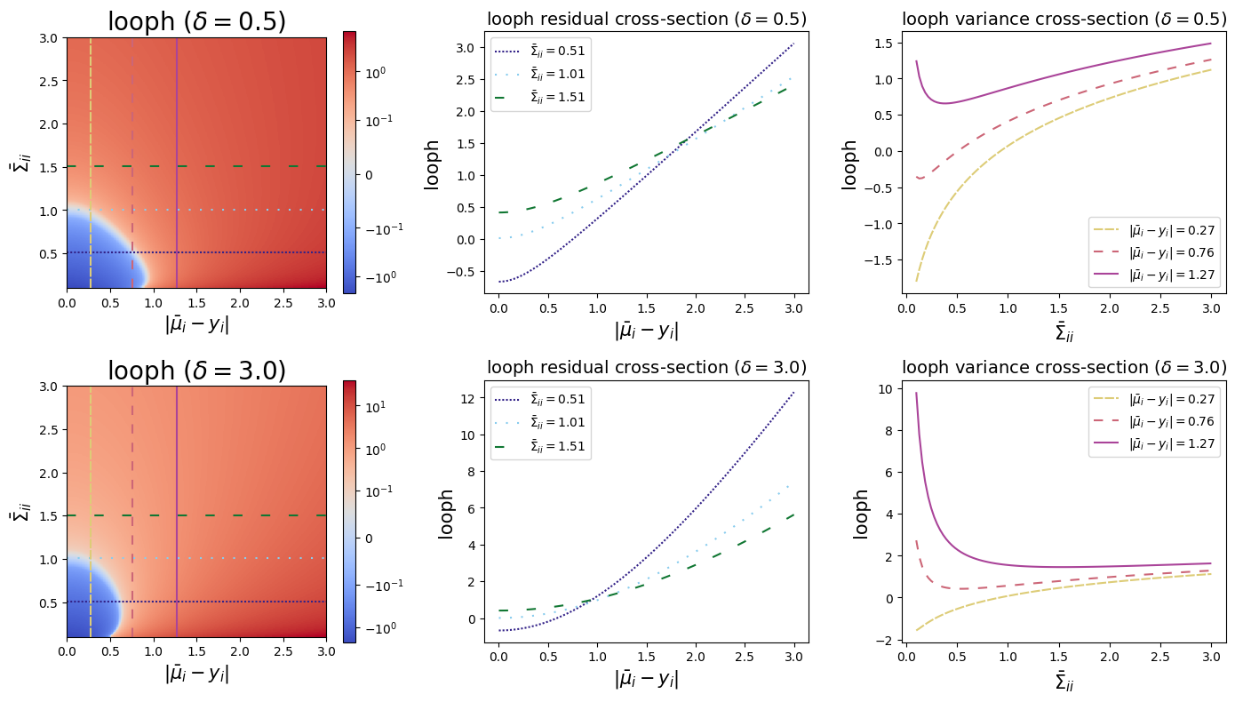
These plots show us that the looph function can exhibit a more exaggerated upward slope where the residual is in the linear component of the pseudo-Huber curve but is not so large that it still outweighs the variance component of the loss. Note that in practice that both pseudo Huber loss functions may require more training iterations to converge than their alternatives.
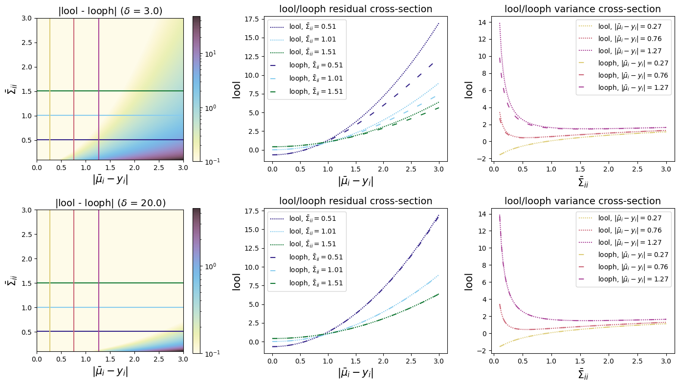
Comparison between lool and looph
Here we compare looph to lool for differing the boundary_scales. We see that, similar to the original pseudo-Huber, the looph also converges to lool as the boundary_scale grows large. Similarly, looph’s loss for a fixed variance becomes linear when \(\frac{(\bar{\mu}_i - y_i)^2}{\Sigma_{ii}}\) exceeds the boundary_scale.
[16]:
compare_boundary_scales = np.array([3.0, 20.0])
compare_loophs = np.array([
    [
        [
            looph_fn(
                ys[i],
                residuals[i],
                variances[variance_count - 1 - j],
                unitary_scale,
                boundary_scale=bs,
            )
            for i in range(residual_count)
        ]
        for j in range(variance_count)
    ]
    for bs in compare_boundary_scales
])

fig, axes = plt.subplots(2, 3, figsize=(14, 4 * len(compare_boundary_scales)))

for i, bs in enumerate(compare_boundary_scales):
    axes[i, 0].set_title(f"|lool - looph| ($\delta$ = {bs})", fontsize=14)
    axes[i, 0].set_ylabel(r"$\bar{\Sigma}_{ii}$", fontsize=15)
    axes[i, 0].set_xlabel(r"$\vert \bar{\mu}_i - y_i \vert$", fontsize=15)
    im = axes[i, 0].imshow(
        np.abs(lools - compare_loophs[i, :, :]), extent=[mmin, mmax, smin, smax], cmap="cb.iris", norm=LogNorm(1e-1)
    )
    fig.colorbar(im, ax=axes[i, 0])
    axes[i, 0].plot(residuals, variance_count * [variance_vis_points[0][1]], color=colors[0], linestyle=linestyles[-1])
    axes[i, 0].plot(residuals, variance_count * [variance_vis_points[1][1]], color=colors[1], linestyle=linestyles[-1])
    axes[i, 0].plot(residuals, variance_count * [variance_vis_points[2][1]], color=colors[2], linestyle=linestyles[-1])
    axes[i, 0].plot(residual_count * [residual_vis_points[0][1]], variances, color=colors[3], linestyle=linestyles[-1])
    axes[i, 0].plot(residual_count * [residual_vis_points[1][1]], variances, color=colors[4], linestyle=linestyles[-1])
    axes[i, 0].plot(residual_count * [residual_vis_points[2][1]], variances, color=colors[5], linestyle=linestyles[-1])

    axes[i, 1].set_title("lool/looph residual cross-section", fontsize=14)
    axes[i, 1].set_ylabel("lool", fontsize=15)
    axes[i, 1].set_xlabel(r"$\vert \bar{\mu}_i - y_i \vert$", fontsize=15)
    axes[i, 1].plot(
        residuals,
        lools[variance_vis_points[0][0], :],
        color=colors[0],
        linestyle=linestyles[0],
        label=r"lool, $\bar{\Sigma}_{ii} = $" + f"{variance_vis_points[0][1]:.2f}",
    )
    axes[i, 1].plot(
        residuals,
        lools[variance_vis_points[1][0], :],
        color=colors[1],
        linestyle=linestyles[0],
        label=r"lool, $\bar{\Sigma}_{ii} = $" + f"{variance_vis_points[1][1]:.2f}",
    )
    axes[i, 1].plot(
        residuals,
        lools[variance_vis_points[2][0], :],
        color=colors[2],
        linestyle=linestyles[0],
        label=r"lool, $\bar{\Sigma}_{ii} = $" + f"{variance_vis_points[2][1]:.2f}",
    )
    axes[i, 1].plot(
        residuals,
        compare_loophs[i, variance_vis_points[0][0], :],
        color=colors[0],
        linestyle=linestyles[2],
        label=r"looph, $\bar{\Sigma}_{ii} = $" + f"{variance_vis_points[0][1]:.2f}",
    )
    axes[i, 1].plot(
        residuals,
        compare_loophs[i, variance_vis_points[1][0], :],
        color=colors[1],
        linestyle=linestyles[2],
        label=r"looph, $\bar{\Sigma}_{ii} = $" + f"{variance_vis_points[1][1]:.2f}",
    )
    axes[i, 1].plot(
        residuals,
        compare_loophs[i, variance_vis_points[2][0], :],
        color=colors[2],
        linestyle=linestyles[2],
        label=r"looph, $\bar{\Sigma}_{ii} = $" + f"{variance_vis_points[2][1]:.2f}",
    )
    axes[i, 1].legend()

    axes[i, 2].set_title("lool/looph variance cross-section", fontsize=14)
    axes[i, 2].set_ylabel("lool", fontsize=15)
    axes[i, 2].set_xlabel(r"$\bar{\Sigma}_{ii}$", fontsize=15)
    axes[i, 2].plot(
        variances,
        np.flip(lools[:, residual_vis_points[0][0]]),
        color=colors[3],
        linestyle=linestyles[0],
        label=r"lool, $\vert \bar{\mu}_i - y_i \vert = $" + f"{residual_vis_points[0][1]:.2f}",
    )
    axes[i, 2].plot(
        variances,
        np.flip(lools[:, residual_vis_points[1][0]]),
        color=colors[4],
        linestyle=linestyles[0],
        label=r"lool, $\vert \bar{\mu}_i - y_i \vert = $" + f"{residual_vis_points[1][1]:.2f}",
    )
    axes[i, 2].plot(
        variances,
        np.flip(lools[:, residual_vis_points[2][0]]),
        color=colors[5],
        linestyle=linestyles[0],
        label=r"lool, $\vert \bar{\mu}_i - y_i \vert = $" + f"{residual_vis_points[2][1]:.2f}",
    )
    axes[i, 2].plot(
        variances,
        np.flip(compare_loophs[i, :, residual_vis_points[0][0]]),
        color=colors[3],
        linestyle=linestyles[2],
        label=r"looph, $\vert \bar{\mu}_i - y_i \vert = $" + f"{residual_vis_points[0][1]:.2f}",
    )
    axes[i, 2].plot(
        variances,
        np.flip(compare_loophs[i, :, residual_vis_points[1][0]]),
        color=colors[4],
        linestyle=linestyles[2],
        label=r"looph, $\vert \bar{\mu}_i - y_i \vert = $" + f"{residual_vis_points[1][1]:.2f}",
    )
    axes[i, 2].plot(
        variances,
        np.flip(compare_loophs[i, :, residual_vis_points[2][0]]),
        color=colors[5],
        linestyle=linestyles[2],
        label=r"looph, $\vert \bar{\mu}_i - y_i \vert = $" + f"{residual_vis_points[2][1]:.2f}",
    )
    axes[i, 2].legend()

plt.tight_layout()
plt.show()